3.3.5. Correct both radial distortion and perspective distortion
The following workflow shows how to use Discorpy to correct both radial distortion and perspective distortion from a dot-pattern image (Fig. 3.3.5.1 (a)) shared on Jerome Kieffer’s github page. The image suffers both types of distortions.
Load the image, segment the dots (Fig. 3.3.5.1 (b)), group them into lines (Fig. 3.3.5.2), and check the residual of the distorted points (Fig. 3.3.5.3).
import numpy as np
import matplotlib.pyplot as plt
import discorpy.losa.loadersaver as losa
import discorpy.prep.preprocessing as prep
import discorpy.proc.processing as proc
import discorpy.post.postprocessing as post

# Initial parameters
file_path = "../../data/dot_pattern_06.jpg"
output_base = "E:/output_demo_05/"
num_coef = 4  # Number of polynomial coefficients
mat0 = losa.load_image(file_path) # Load image
(height, width) = mat0.shape

# Normalize background
mat1 = prep.normalization_fft(mat0, sigma=20)
# Segment dots
threshold = prep.calculate_threshold(mat1, bgr="bright", snr=1.5)
mat1 = prep.binarization(mat1, thres=threshold)
losa.save_image(output_base + "/segmented_dots.jpg", mat1)

# Calculate the median dot size and distance between them.
(dot_size, dot_dist) = prep.calc_size_distance(mat1)
# Calculate the slopes of horizontal lines and vertical lines.
hor_slope = prep.calc_hor_slope(mat1)
ver_slope = prep.calc_ver_slope(mat1)
print("Horizontal slope: {0}. Vertical slope: {1}".format(hor_slope, ver_slope))

# Group dots into lines.
list_hor_lines0 = prep.group_dots_hor_lines(mat1, hor_slope, dot_dist,
                                            ratio=0.3, num_dot_miss=2,
                                            accepted_ratio=0.6)
list_ver_lines0 = prep.group_dots_ver_lines(mat1, ver_slope, dot_dist,
                                            ratio=0.3, num_dot_miss=2,
                                            accepted_ratio=0.6)

# Save output for checking
losa.save_plot_image(output_base + "/horizontal_lines.png", list_hor_lines0, height, width)
losa.save_plot_image(output_base + "/vertical_lines.png", list_ver_lines0, height, width)
list_hor_data = post.calc_residual_hor(list_hor_lines0, 0.0, 0.0)
list_ver_data = post.calc_residual_ver(list_ver_lines0, 0.0, 0.0)
losa.save_residual_plot(output_base + "/hor_residual_before_correction.png", list_hor_data,
                      height, width)
losa.save_residual_plot(output_base + "/ver_residual_before_correction.png", list_ver_data,
                      height, width)
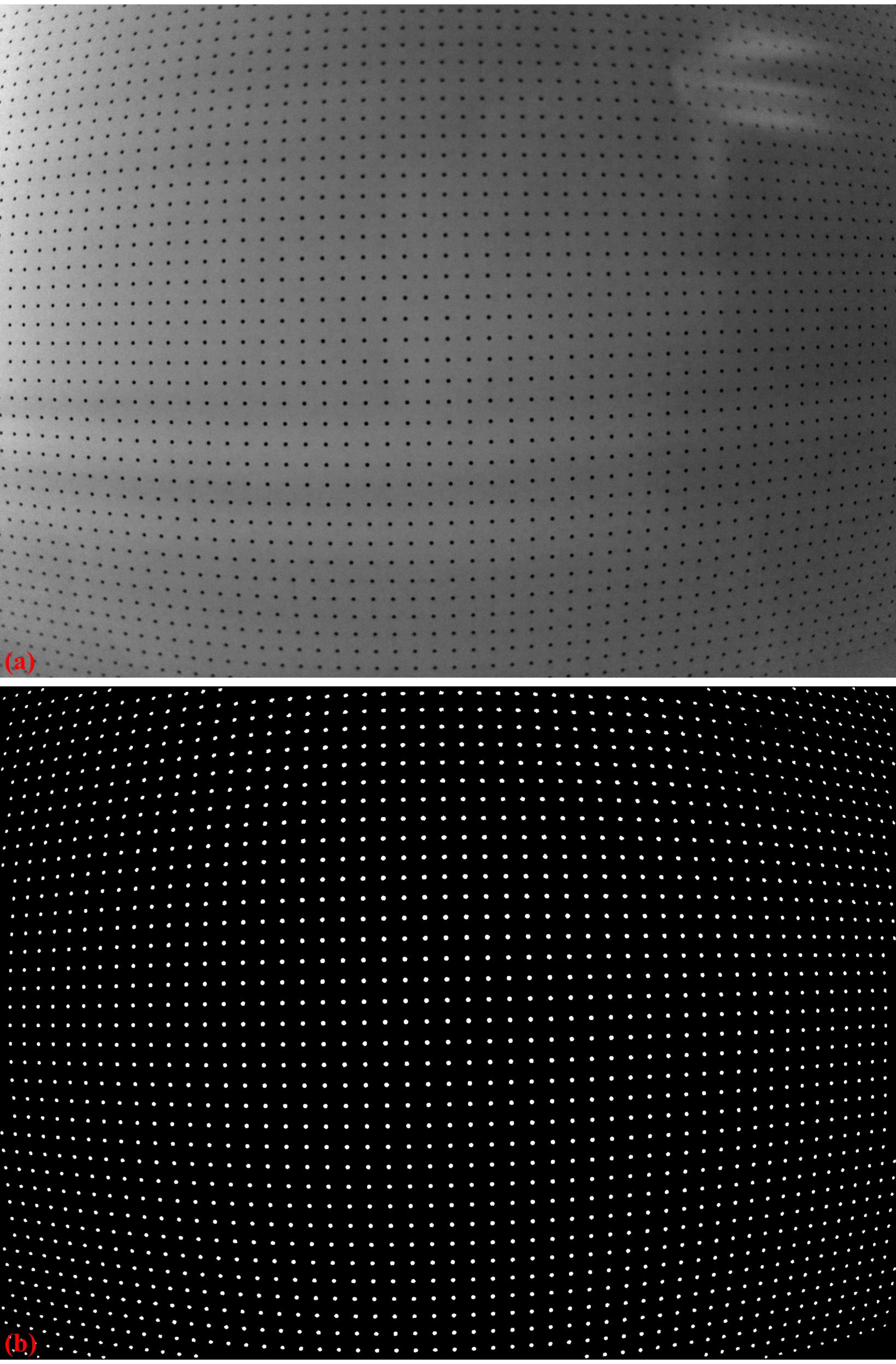
Fig. 3.3.5.1 . (a) Calibration image. (b) Binarized image.
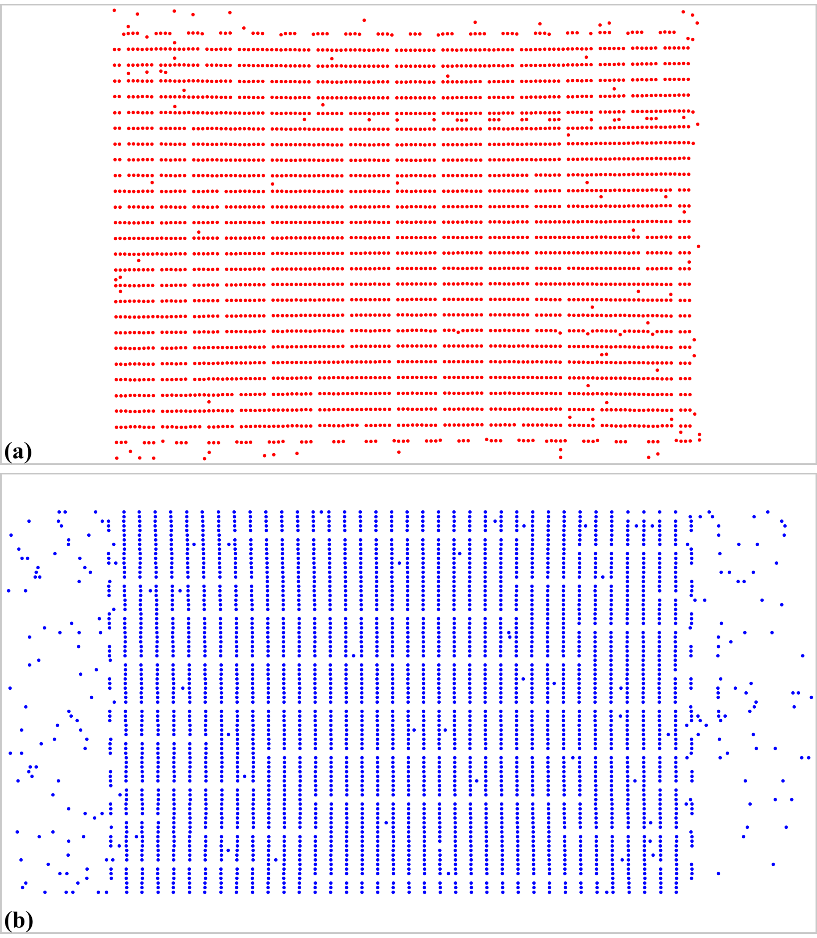
Fig. 3.3.5.2 Grouped points. (a) Horizontal lines. (b) Vertical lines.
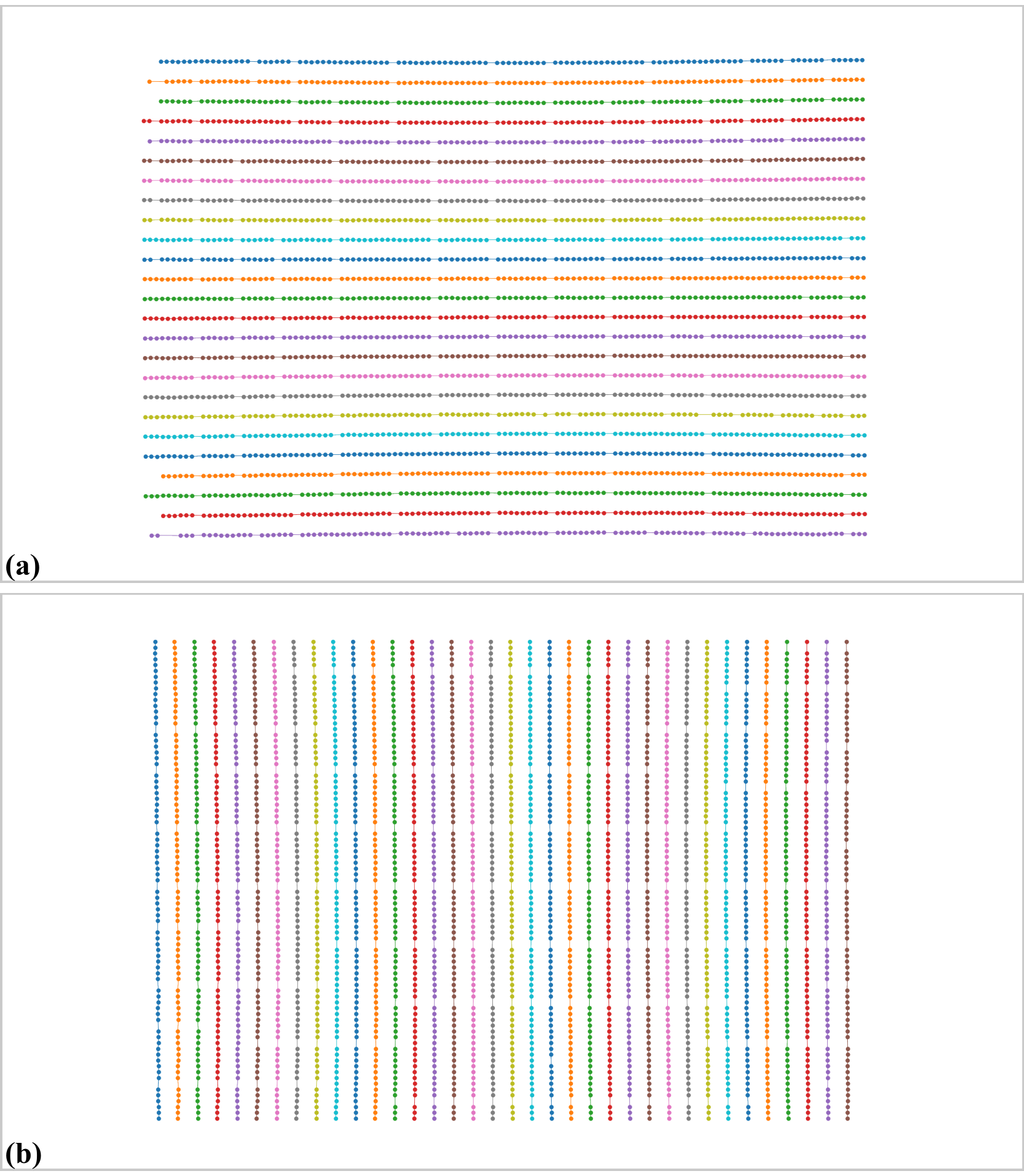
Fig. 3.3.5.3 Residual of distorted points. (a) Horizontal lines. (b) Vertical lines.
Perspective distortion can be detected by using coefficients of parabolic fits to the horizontal lines and vertical lines (Fig. 3.3.5.4) as presented in the method section. The effect of perspective distortion is corrected by adjusting these parabolic coefficients (Fig. 3.3.5.5). Then, they will be used for the step of determining parameters of the radial distortion model.
# Optional: for checking perspective distortion
(xcen_tmp, ycen_tmp) = proc.find_cod_bailey(list_hor_lines0, list_ver_lines0)
list_hor_coef = proc._para_fit_hor(list_hor_lines0, xcen_tmp, ycen_tmp)[0]
list_ver_coef = proc._para_fit_ver(list_ver_lines0, xcen_tmp, ycen_tmp)[0]
# Optional: plot the results
plt.figure(0)
plt.plot(list_hor_coef[:, 2], list_hor_coef[:, 0], "-o")
plt.plot(list_ver_coef[:, 2], list_ver_coef[:, 0], "-o")
plt.xlabel("c-coefficient")
plt.ylabel("a-coefficient")

plt.figure(1)
plt.plot(list_hor_coef[:, 2], -list_hor_coef[:, 1], "-o")
plt.plot(list_ver_coef[:, 2], list_ver_coef[:, 1], "-o")
plt.xlabel("c-coefficient")
plt.ylabel("b-coefficient")
plt.show()
# Optional: correct parabola coefficients
hor_coef_corr, ver_coef_corr = proc._generate_non_perspective_parabola_coef(
    list_hor_lines0, list_ver_lines0)[0:2]
# Optional: plot to check the results
plt.figure(0)
plt.plot(hor_coef_corr[:, 2], hor_coef_corr[:, 0], "-o")
plt.plot(ver_coef_corr[:, 2], ver_coef_corr[:, 0], "-o")
plt.xlabel("c-coefficient")
plt.ylabel("a-coefficient")
plt.figure(1)
plt.plot(hor_coef_corr[:, 2], -hor_coef_corr[:, 1], "-o")
plt.plot(ver_coef_corr[:, 2], ver_coef_corr[:, 1], "-o")
plt.xlabel("c-coefficient")
plt.ylabel("b-coefficient")
plt.show()

# Regenerate grid points with the correction of perspective effect.
list_hor_lines1, list_ver_lines1 = proc.regenerate_grid_points_parabola(
    list_hor_lines0, list_ver_lines0, perspective=True)
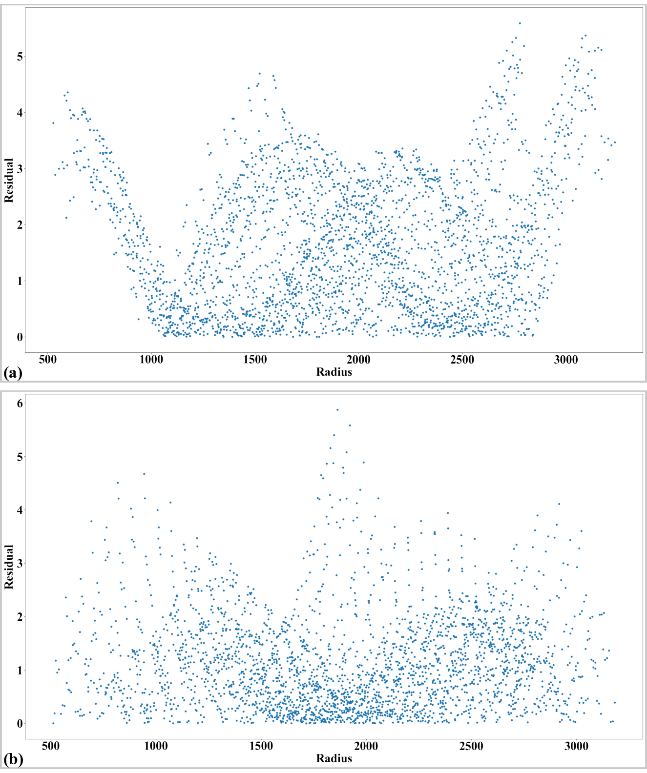
Fig. 3.3.5.4 . (a) Plot of a-coefficients vs c-coefficients of parabolic fits. (b) Plot of b-coefficients vs c-coefficients.
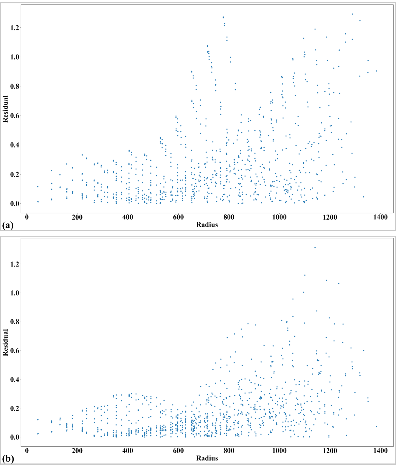
Fig. 3.3.5.5 Parabola coefficients after correction. (a) Plot of a-coefficients vs c-coefficients. (b) Plot of b-coefficients vs c-coefficients.
Parameters of the radial distortion correction are determined and the image is corrected. At this step only radial distortion correction is applied (Fig. 3.3.5.7 (a)). For checking the accuracy of the model, noting that unwarping lines using the backward model is based on optimization [R5] which may result in strong fluctuation if lines are strongly curved. In such case, using the forward model is more reliable.
# Calculate parameters of the radial correction model
(xcenter, ycenter) = proc.find_cod_coarse(list_hor_lines1, list_ver_lines1)
list_fact = proc.calc_coef_backward(list_hor_lines1, list_ver_lines1,
                                    xcenter, ycenter, num_coef)
losa.save_metadata_txt(output_base + "/coefficients_radial_distortion.txt",
                     xcenter, ycenter, list_fact)
print("X-center: {0}. Y-center: {1}".format(xcenter, ycenter))
print("Coefficients: {0}".format(list_fact))

# Regenerate the lines without perspective correction for later use.
list_hor_lines2, list_ver_lines2 = proc.regenerate_grid_points_parabola(
    list_hor_lines0, list_ver_lines0, perspective=False)

# Unwarp lines using the backward model:
list_uhor_lines = post.unwarp_line_backward(list_hor_lines2, xcenter, ycenter, list_fact)
list_uver_lines = post.unwarp_line_backward(list_ver_lines2, xcenter, ycenter, list_fact)

# Optional: unwarp lines using the forward model.
# list_ffact = proc.calc_coef_forward(list_hor_lines1, list_ver_lines1,
#                                     xcenter, ycenter, num_coef)
# list_uhor_lines = post.unwarp_line_forward(list_hor_lines2, xcenter, ycenter,
#                                            list_ffact)
# list_uver_lines = post.unwarp_line_forward(list_ver_lines2, xcenter, ycenter,
#                                            list_ffact)

# Check the residual of unwarped lines:
list_hor_data = post.calc_residual_hor(list_uhor_lines, xcenter, ycenter)
list_ver_data = post.calc_residual_ver(list_uver_lines, xcenter, ycenter)
losa.save_residual_plot(output_base + "/hor_residual_after_correction.png", list_hor_data,
                      height, width)
losa.save_residual_plot(output_base + "/ver_residual_after_correction.png", list_ver_data,
                      height, width)

# Unwarp the image
mat_rad_corr = post.unwarp_image_backward(mat0, xcenter, ycenter, list_fact)
# Save results
losa.save_image(output_base + "/image_radial_corrected.jpg", mat_rad_corr)
losa.save_image(output_base + "/radial_difference.jpg", mat_rad_corr - mat0)
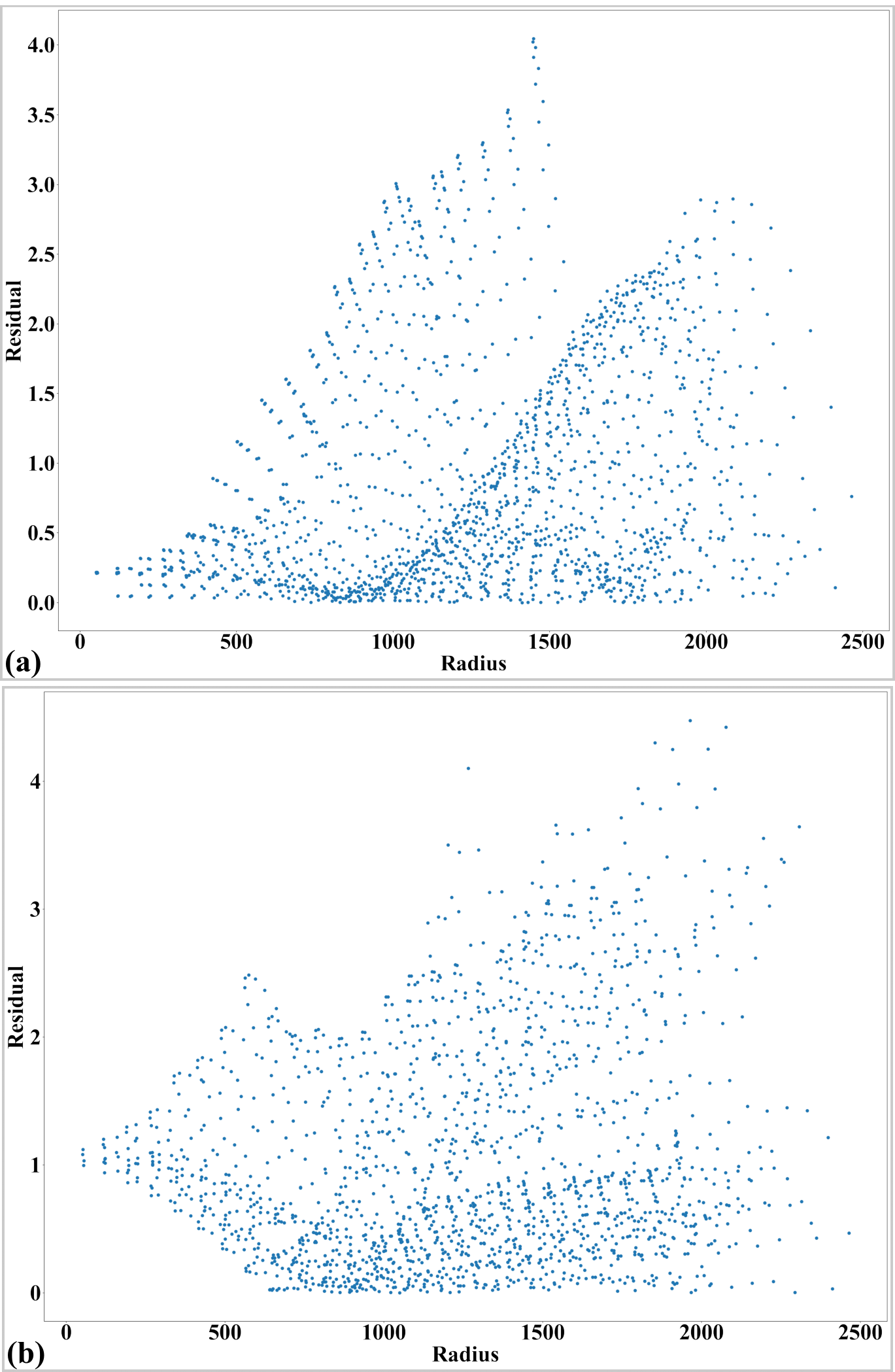
Fig. 3.3.5.6 Residual of unwarped points in the horizontal lines (a) and vertical lines (b). Note that this is from a commercial camera, the accuracy may not be at sub-pixel as compared to scientific cameras used in demo 1-4.
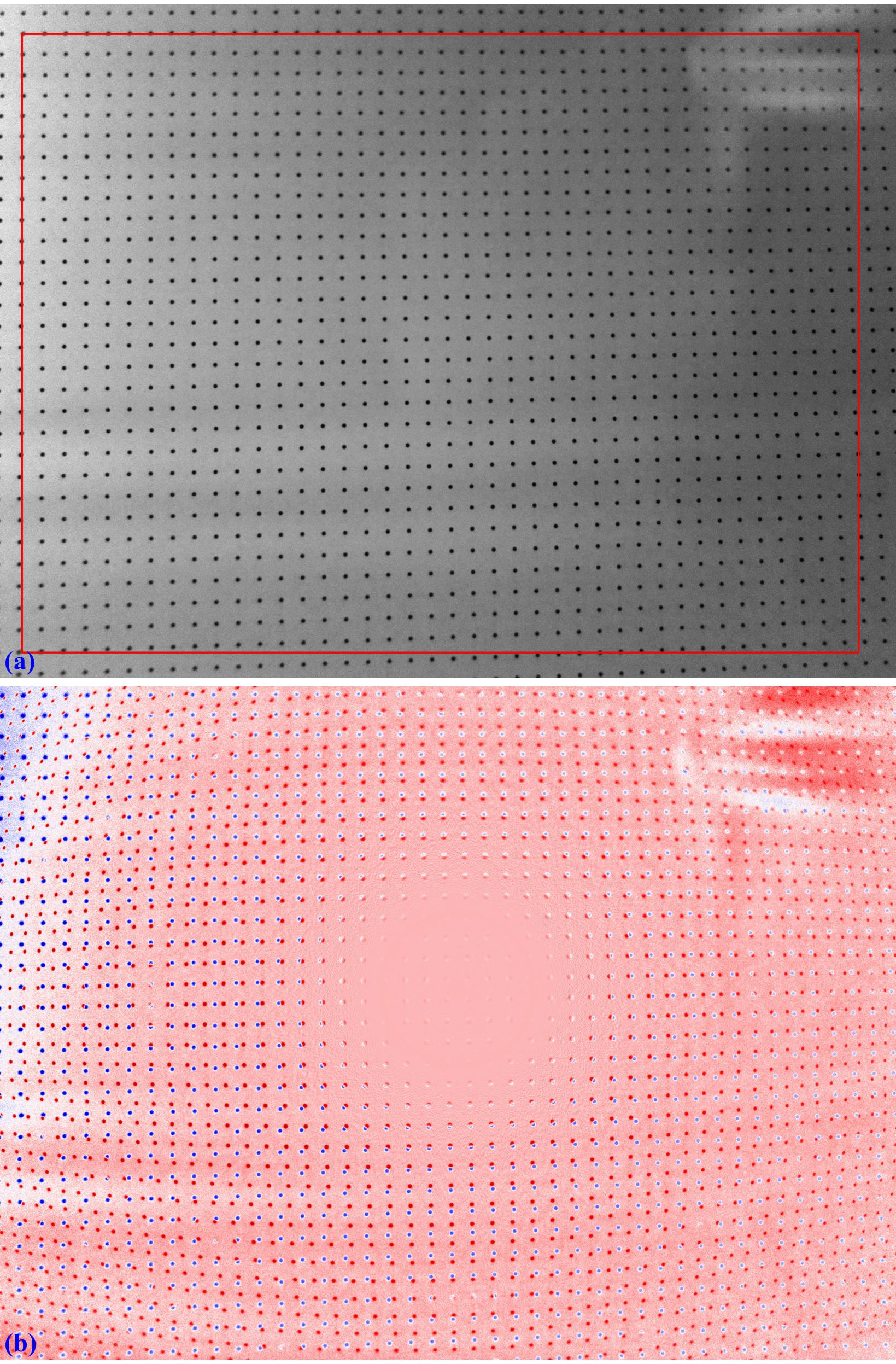
Fig. 3.3.5.7 . (a) Unwarped image where perspective distortion can be seen. (b) Difference between image in Fig. 3.3.5.7 (a) and image in Fig. 3.3.5.1 (a).
Perspective distortion can be caused by the calibration-object-plane not parallel to the camera-sensor plane. In such case, determining the radial distortion coefficients is enough. However, if the distortion is caused by the lens-plane (tangential distortion), we need to correct for this type of distortion, too. This is straightforward using Discorpy’s API.
# Generate source points and target points to calculate coefficients of a perspective model
source_points, target_points = proc.generate_source_target_perspective_points(list_uhor_lines, list_uver_lines,
                                                                              equal_dist=True, scale="mean",
                                                                              optimizing=False)
# Calculate perspective coefficients:
pers_coef = proc.calc_perspective_coefficients(source_points, target_points, mapping="backward")
image_pers_corr = post.correct_perspective_image(mat_rad_corr, pers_coef)
# Save results
np.savetxt(output_base + "/perspective_coefficients.txt", np.transpose([pers_coef]))
losa.save_image(output_base + "/image_radial_perspective_corrected.jpg", image_pers_corr)
losa.save_image(output_base + "/perspective_difference.jpg", image_pers_corr - mat_rad_corr)

Fig. 3.3.5.8 Image showing source-points and targets-points used to calculate perspective-distortion coefficients
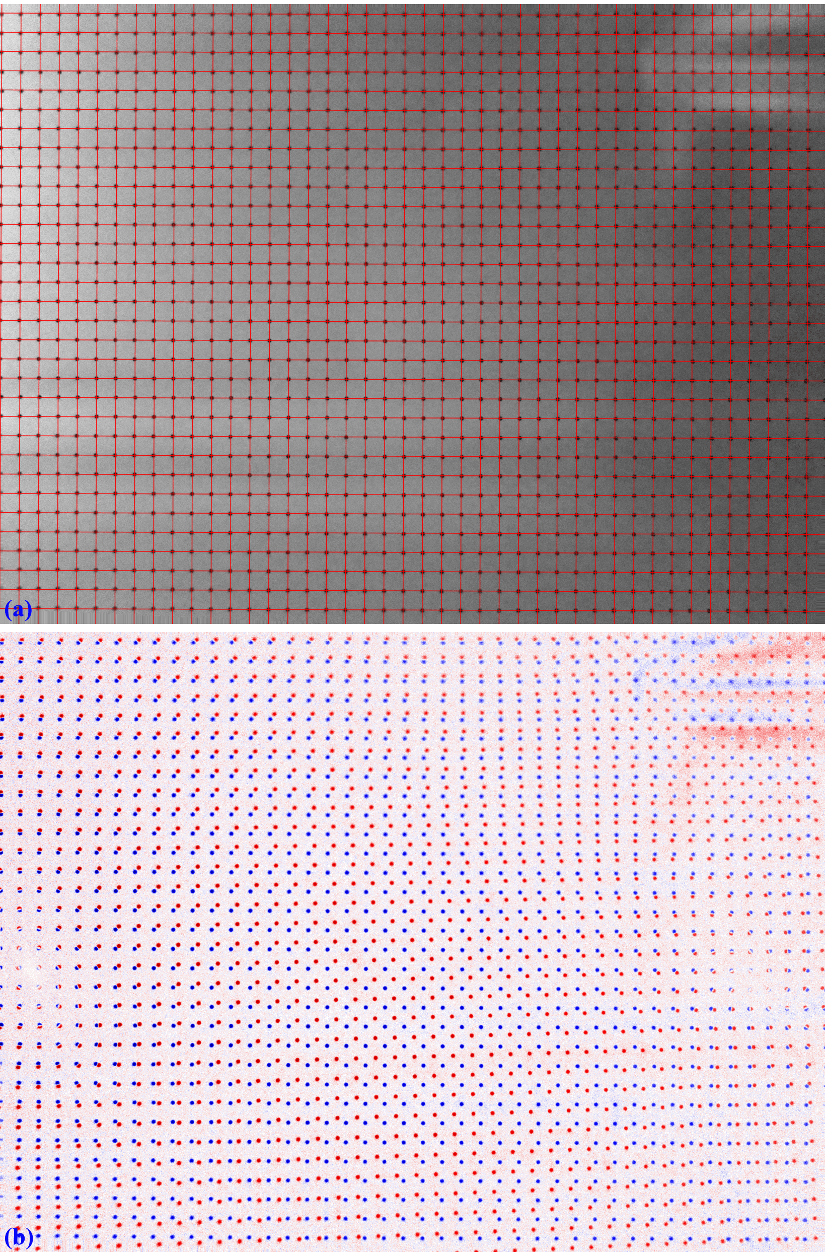
Fig. 3.3.5.9 . (a) Perspective corrected image. (b) Difference between image in Fig. 3.3.5.9 (a) and image in Fig. 3.3.5.7 (a).
Click here to download the Python codes.