2.2. Methods for correcting distortions
2.2.1. Introduction
For correcting radial and/or perspective distortion, we need to know a model to map between distorted space and undistorted space. Mapping from the undistorted space to the distorted space is the forward mapping (Fig. 2.2.1.1). The reverse process is the backward mapping or inverse mapping (Fig. 2.2.1.2).

Fig. 2.2.1.1 Forward mapping.
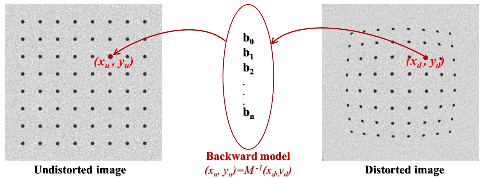
Fig. 2.2.1.2 Backward mapping.
There are many models which can be chosen from literature [R1, R2, R3] such as polynomial, logarithmic, field-of-view, or matrix-based models to describe the relationship between the undistorted space and distorted space. Some models were proposed for only one type of distortion while others are for both distortion types including the location of the optical center. From a selected model, we can find a practical approach to calculate the parameters of this model.
To calculate parameters of a distortion model, we have to determine the coordinates of reference points in the distorted space and their positions in the undistorted space, correspondingly. Reference points can be extracted using an image of a calibration object giving a line or dot-pattern image (Fig. 2.2.1.1), which is distorted. Using conditions that lines of these points must be straight, equidistant, parallel, or perpendicular we can estimate the locations of these reference-points in the undistorted space with high-accuracy.
Among many models for characterizing radial distortion, the polynomial model is versatile enough to correct both small-to-medium distortion with sub-pixel accuracy [Haneishi], [C1] and strong distortion such as fisheye effect [Basu]. For a comprehensive overview of radial distortion correction methods, readers are recommended to refer to these review articles [Hughes-2008], [Hughes-2010], [R2]. When perspective distortion and optical center offset are present, radial distortion can be calibrated using two main approaches. One approach is iterative optimization, which uses a cost function to ensure that corrected lines in the undistorted image appear straight [Devernay]. Although it requires only a single calibration image, this method is computationally expensive and does not always guarantee convergence. The other approach relies on multiple calibration images to estimate all distortion parameters, as implemented in OpenCV. However, its accuracy is limited because the polynomial model uses only even-order terms [Zhang]. Therefore, a method for calibrating radial distortion in the presence of other distortions that achieves high accuracy using only a single calibration image is both practical and crucially needed.
Discorpy is the Python implementation of radial distortion correction methods presented in [C1]. These methods employ polynomial models and use a calibration image for calculating coefficients of the models where the optical center is determined independently. The reason of using these models and a calibration image is to achieve sub-pixel accuracy as strictly required by parallel-beam tomography systems. The methods were developed and used internally at the beamline I12 and I13, Diamond Light Source-UK, as Mathematica codes. In 2018, they were converted to Python codes and packaged as open-source software under the name Vounwarp. The name was changed to Discorpy in 2021. At the beginning of the software development, only methods for radial distortion characterization were provided as the optical design of the detection system at I12 features a plug-and-play scintillator that can be swapped with a dot-target, enabling the removal of perspective distortion. However, in the detection system at I13, replacing the scintillator with a visible light dot-target is not practical. Instead, an X-ray dot target has been used. The main disadvantage of this approach is that it is difficult to align the target to minimize perspective distortion to an ignorable level. To address this problem, starting with version 1.4 of Discorpy, algorithms for perspective characterization and correction based on [R3] has been developed and added to software.
The inclusion of perspective correction independent of radial distortion correction was a significant development, enabling broader applications of Discorpy beyond scientific purposes. Considering that previous algorithms in Discorpy were primarily focused on calibrating small-to-medium distortions, methods for calibrating strong radial distortion, known as fisheye distortion, have been developed, published in [C2], and added to Discorpy from version 1.7. With this new development, Discorpy and its algorithms stand out for their capability of independently characterizing both distortion types - radial distortion and perspective distortion of varying strengths - with high accuracy using a single calibration image. This makes Discorpy a practical tool for a wide range of imaging applications.
2.2.2. Extracting reference-points from a calibration image
The purpose of a calibration-image (Fig. 2.2.2.1 (a,b,c)) is to provide reference-points (Fig. 2.2.2.1 (d)) which can be extracted from the image using some image processing techniques. As shown in Fig. 2.2.2.1, there are a few calibration-images can be used in practice. A dot-pattern image (Fig. 2.2.2.1 (a)) is the easiest one to process because we just need to segment the dots and calculate the center-of-mass of each dot. For a line-pattern image (Fig. 2.2.2.1 (b)), a line-detection technique is needed. Points on the detected lines or the crossing points between these lines can be used as reference-points. For a chessboard image (Fig. 2.2.2.1 (c)), one can employ some corner-detection techniques or apply a gradient filter to the image and use a line-detection technique.
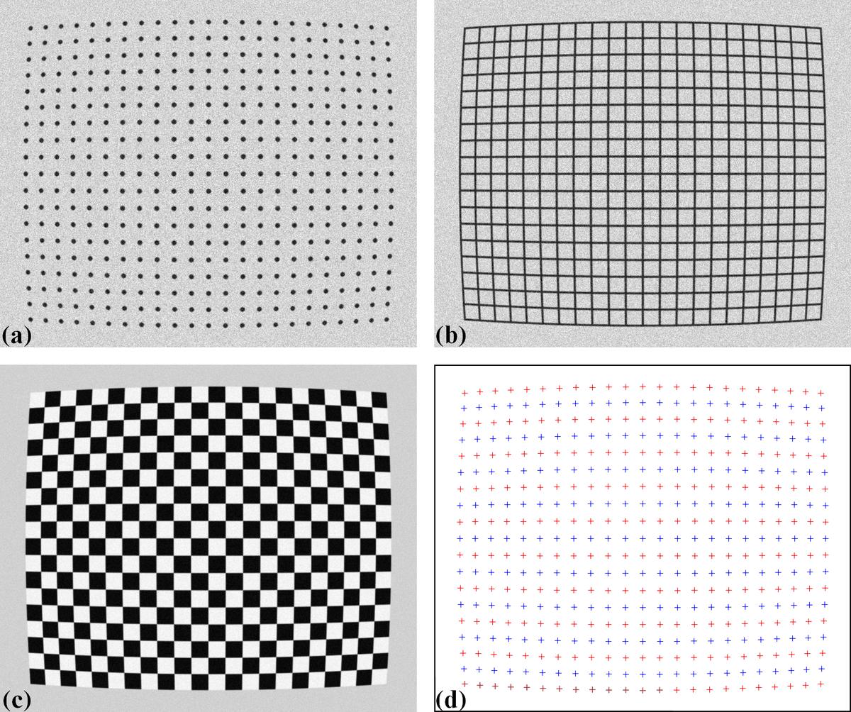
Fig. 2.2.2.1 (a) Dot-pattern image. (b) Line-pattern image. (c) Chessboard image. (d) Extracted reference-points from the image (a),(b), and (c).
In practice, acquired calibration images do not always look nice as shown in Fig. 2.2.2.1. Some are very challenging to get reference-points. The following sub-sections present practical approaches to process calibration images in such cases:
2.2.3. Grouping reference-points into horizontal lines and vertical lines
Different techniques of calculating parameters of a distortion-model use reference-points differently. The techniques [C1, R4] implemented in Discorpy group reference-points into horizontal lines and vertical lines (Fig. 2.2.3.1), represent them by the coefficients of parabolic fits, and use these coefficients for calculating distortion-parameters.
Fig. 2.2.3.1 (a) Points are grouped into horizontal lines. (b) Points are grouped into vertical lines.
The grouping step is critical in data processing workflow. It dictates the performance of other methods down the line. In Discorpy, the grouping method works by searching the neighbours of a point to decide if they belong to the same group or not. The search window is defined by the distance between two nearest reference-points, the slope of the grid, the parameter R, and the acceptable number of missing points. Depending on the quality of a calibration image, users may need to tweak parameters of pre-processing methods and/or the grouping method to get the best results (Fig. 2.2.3.2).
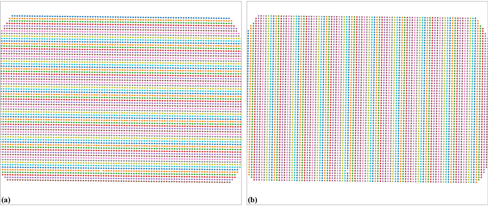
Fig. 2.2.3.2 (a) Points extracted from a calibration image including unwanted points. (b) Results of applying the grouping method to points in (a).
The introduced method works well for small-to-medium distortions where lines are not strongly curved. However, for fisheye images, where lines are significantly curved, using the slope (orientation) of the grid to guide the search is not effective. To address this problem, a different approach has been developed [C2], where points are grouped from the middle of the image outward, guided by a polynomial fit to locate nearby points. The process includes two steps: first, in the horizontal direction, points around the center of the image, where distortion is minimal, are grouped line by line using the previous method. For each group of points, a parabolic fit is applied. The search window then moves to the next slab (left and right from the center) and selects points close to the fitted parabola. The parabolic fit is then updated to include the newly grouped points. This search window continues moving to both sides until the entire image is covered (Fig. 2.2.3.3).
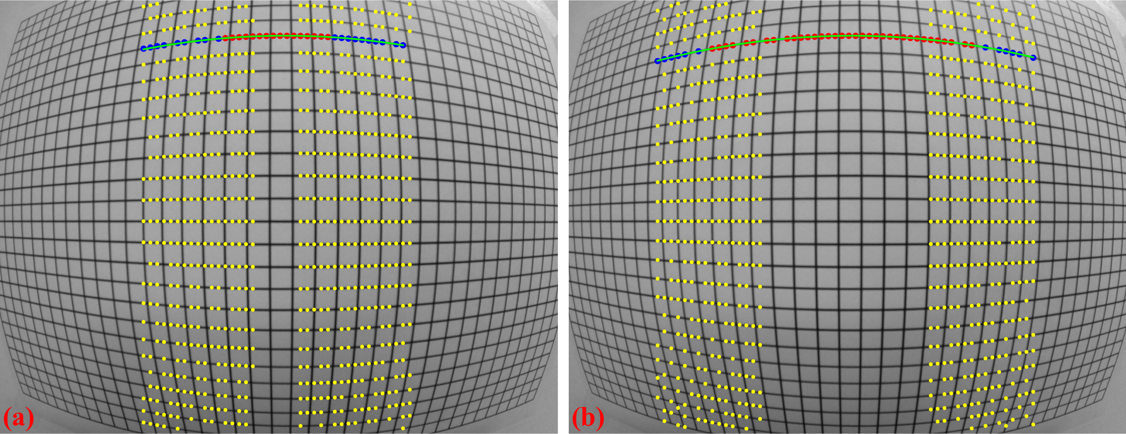
Fig. 2.2.3.3 Demonstration of the grouping method for strongly curved lines: (a) Initial search window, (b) Next search window.
After points are grouped line-by-line, the coordinates of points on each group are fitted to parabolas in which horizontal lines are represented by
and vertical lines by
where \(i\), \(j\) are the indices of the horizontal and vertical lines, respectively. Noting that the origin of \(x\) and \(y\) corresponds to image coordinate system, i.e. the top-left corner of the image.
2.2.4. Calculating the optical center of radial distortion
If there is no perspective distortion, the center of distortion (COD) is determined as explained in Fig. 2.2.4.1 where (\({x_0}\), \({y_0}\)) is the average of the axis intercepts \(c\) of two parabolas between which the coefficient \(a\) changes sign. The slopes of the red and green line are the average of the \(b\) coefficients of these parabolas.
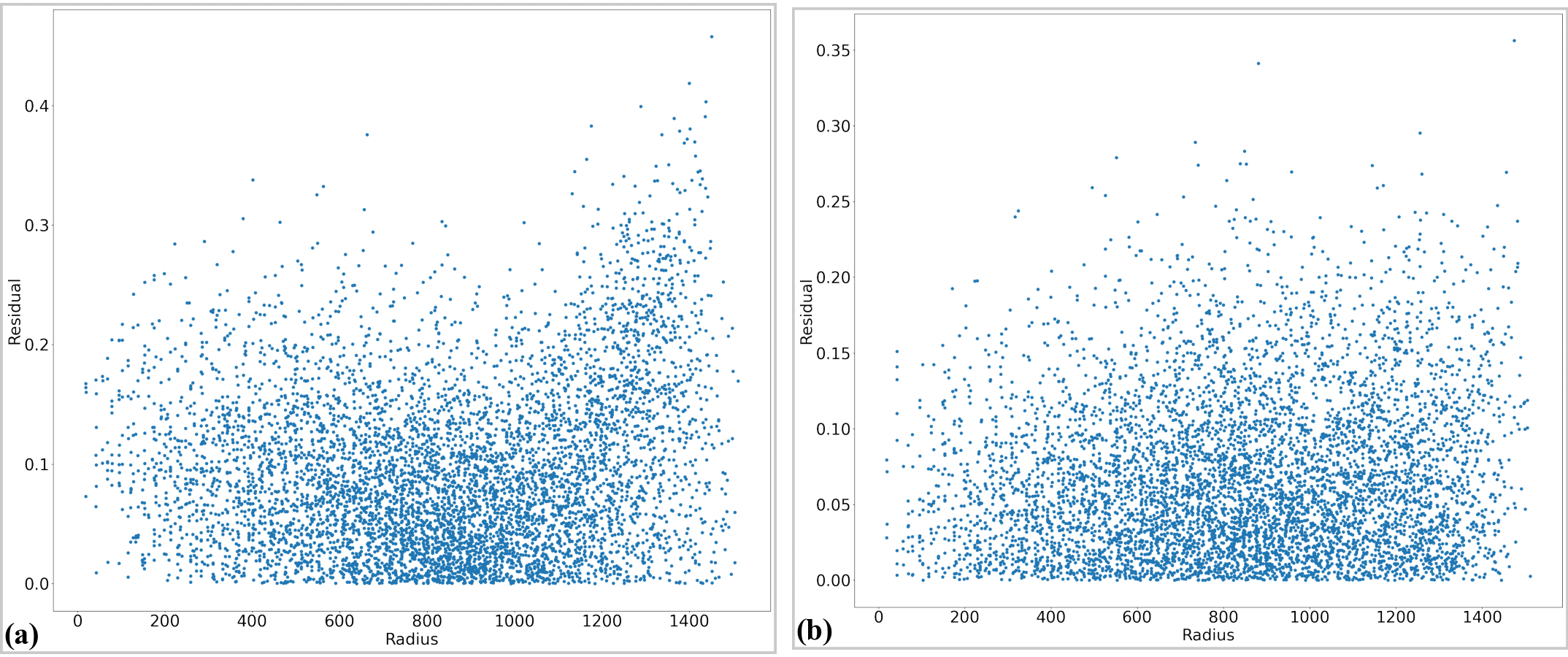
Fig. 2.2.4.1 Intersection between the red and the green line is the CoD.
For calculating the COD with high accuracy, Discorpy implements two methods. One approach is described in details in [R4] where the linear fit is applied to a list of (\(a\), \(c\)) coefficients in each direction to find x-center and y-center of the distortion. Another approach, which is slower but more accurate, is shown in [C1]. The technique varies the COD around the coarse-estimated COD and calculate a corresponding metric (Fig. 2.2.4.2). The best COD is the one having the minimum metric. This approach, however, is sensitive to perspective distortion. In practice, it is found that the coarse COD is accurate enough.
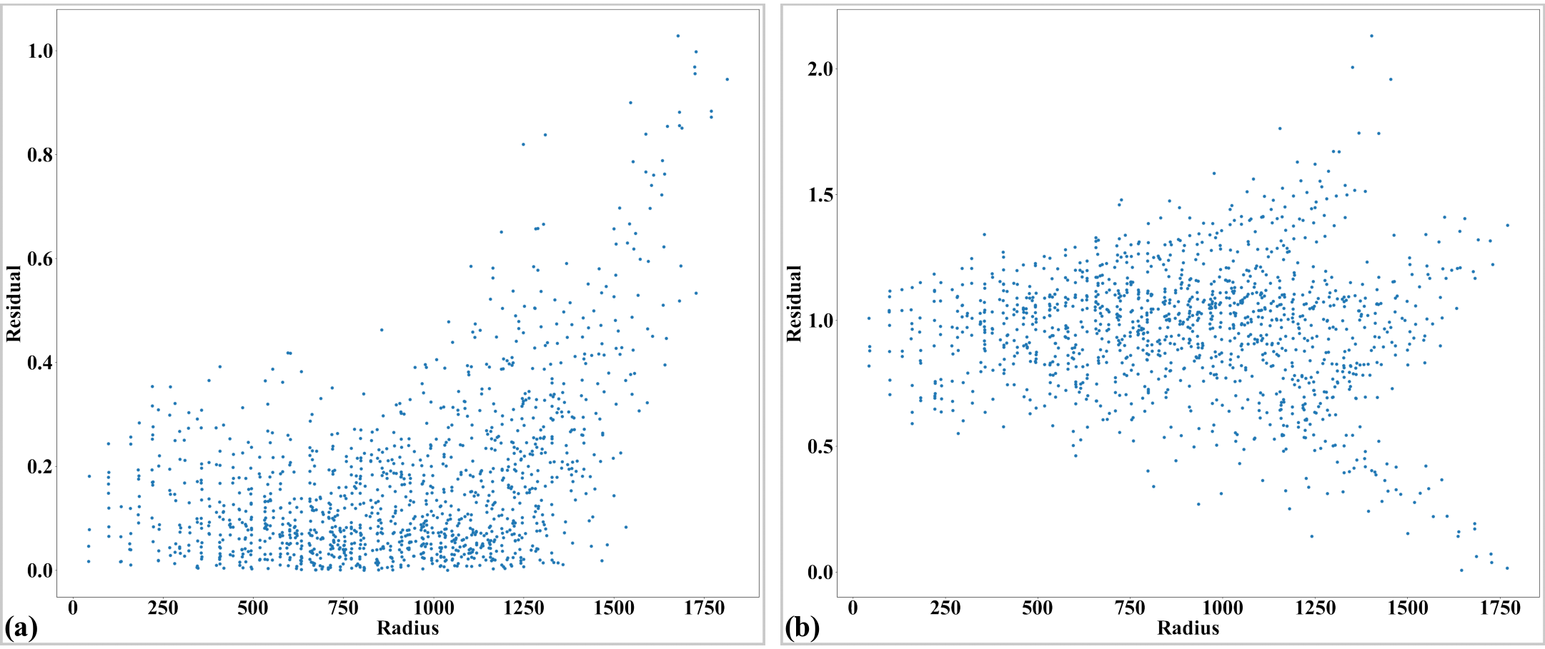
Fig. 2.2.4.2 Metric map of the CoD search.
For cases where perspective distortion is present and radial distortion is not strong, methods proposed in [R4] can be used. However, for strong radial distortion, two approaches have been developed [C2]. These methods is based on the idea of using vanishing points [Hughes] formed by the intersections of distorted line. However, unlike the approach described in that article, the method developed for Discorpy uses parabola fitting instead of circular fitting, and it does not attempt to locate four vanishing points. Instead, the first approach involves finding the intersection points between parabolas with opposite signs of the \(a\)-coefficient at the same orientation, e.g., horizontal parabolas. A linear fit is then applied to these points (Fig. 2.2.4.3). The same process is repeated for vertical parabolas. The intersection of the two fitted lines provides the distortion center. This method works well only for barrel radial distortion.

Fig. 2.2.4.3 Demonstration of the method for finding the distortion center using the vanishing points
For broader applicability where perspective distortion of calibration image is strong, the second approach is as follows: for each orientation, e.g., horizontal direction, the parabola with the absolute minimum \(a\)-coefficient is identified, then the intersection points between this parabola and the rest are calculated. A linear fit is applied to these points. The same routine is repeated for vertical direction parabolas. The intersection points of these two fitted lines determine the calculated center. This entire routine is repeated two or three times to refine the calculated center further by combining it with perspective distortion correction, as will be shown in the next section.
2.2.5. Correcting perspective effect
In practice, the target object used for acquiring a calibration image is often not aligned parallel to the sensor-plane. This causes perspective distortion in the acquired image, which affects the accuracy of the calculated model for radial distortion. Perspective distortion can be detected by analyzing the parabolic coefficients of lines [R4] where the origin of the coordinate system is shifted to the COD, calculated by the approaches shown in above ([R4] or [C2]), before the parabola fitting. Fig. 2.2.5.1 (a) shows the plot of \(a\)-coefficients against \(c\)-coefficients for horizontal lines (Eq. (2.2.3.1)) and vertical lines (Eq. (2.2.3.2)). If there is perspective distortion, the slopes of straight lines fitted to the plotted data are different. The other consequence is that \(b\)-coefficients vary against \(c\)-coefficients instead of staying the same (Fig. 2.2.5.1 (b)). For comparison, corresponding plots of parabolic coefficients for the case of no perspective-distortion are shown in Fig. 2.2.5.2.
Fig. 2.2.5.1 Effects of perspective distortion to parabolic coefficients. (a) Between \(a\) and \(c\)-coefficients. (b) Between \(b\) and \(c\)-coefficients. Noting that the sign of the \(b\)-coefficients for vertical lines has been reversed to match the sign of the horizontal lines.
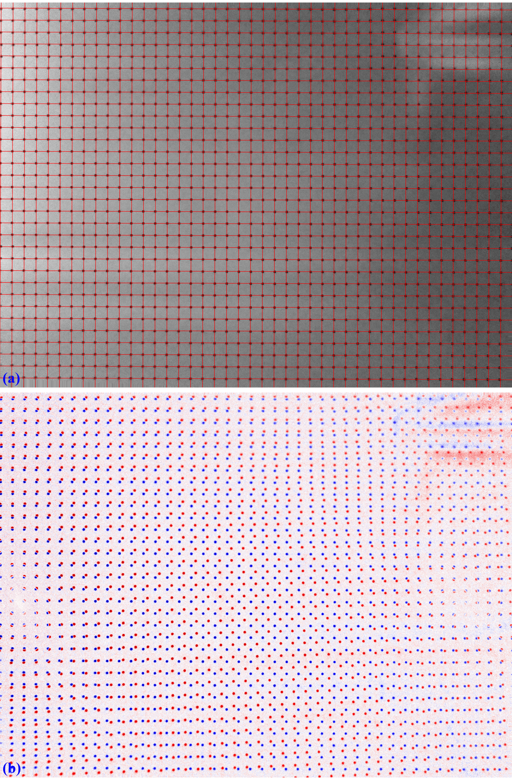
Fig. 2.2.5.2 (a) Corresponding to Fig. 2.2.5.1 (a) without perspective distortion. (b) Corresponding to Fig. 2.2.5.1 (b) without perspective distortion.
To calibrate radial distortion, perspective distortion must be corrected first. This can be achieved in two ways. In the first approach, the coefficients of the parabolic fit are adjusted. Specifically, the \(a\)- and \(c\)- coefficients of parabolas in one direction (e.g., horizontal) are corrected using a ratio calculated as the division between the average of the differences of \(c\)-coefficients in the other direction (vertical) and those in the same direction (horizontal). The \(b\)-coefficient is simply taken as the value at the intersection of the fitted lines, as shown in Fig. 2.2.5.1 (b). The grid lines are then regenerated using these updated coefficients. This approach was introduced from Discorpy 1.4 and works well for small-to-medium radial distortion. However, for strong distortion - fisheye image, the graphs of \(a\)-versus-\(c\) coefficients and \(b\)-versus-\(c\) coefficients are not straight, as shown in Fig. 2.2.5.3.
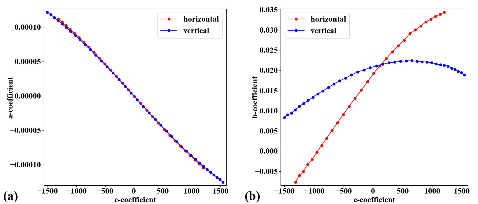
Fig. 2.2.5.3 Effects of perspective distortion on parabolic coefficients of a strongly distorted grid: (a) Relationship between \(a\)- and \(c\)-coefficients, (b) \(b\) and \(c\)-coefficients.
To address this problem, perspective distortion is calibrated using the fact that the representative lines between directions are perpendicular and using the perspective model presented in the next section.
2.2.6. Calculating coefficients of a correction model for perspective distortion
The perspective model is described in [R3] where the forward mapping between a distorted point and an undistorted point are given by
These equations can be rewritten as
which can be formulated as a system of linear equations for n couple-of-points (1 distorted point and its corresponding point in the undistorted space).
For the backward mapping, the coordinates of corresponding points in Eq. (9-13) are simply swapped which results in
To find 8 coefficients in Eq. (2.2.6.5) or Eq. (2.2.6.8), the coordinates of at least 4 couple-of-points are needed where 1 couple-of-points provides 2 equations. If there are more than 4 couple-of-points, a least square method is used to solve the equation. Given the coordinates of distorted points on grid lines, using conditions that lines connecting these points must be parallel, equidistant, or perpendicular we can calculate the coordinates of undistorted points (Fig. 2.2.6.1) correspondingly. Details of this implementation can be found in Discorpy’s API.
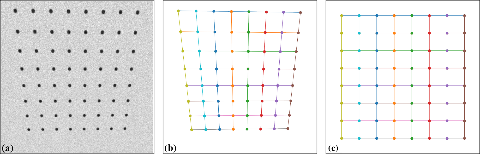
Fig. 2.2.6.1 Demonstration of generating undistorted points from perspective points. (a) Calibration image. (b) Extracted reference-points. (c) Undistorted points generated by using the conditions that lines are parallel in each direction, perpendicular between direction, and equidistant. As the scale between the distorted space and undistorted space are unknown, the distance between lines in the undistorted space can be arbitrarily chosen. Here the mean of distances in the distorted space is used.
The following describes the second approach of correcting perspective effect [C2] from a radial-distortion calibration-image, which calculates the coefficients of the above model and applies correction.
First, the distortion center is determined using the vanishing points approach described in the above section. The coordinates of the reference points are updated by shifting the origin from the top-left corner of the image to the distortion center, and the parabola fit is recalculated using the updated coordinates. Next, the intersection of four lines is found: two in the horizontal direction and two in the vertical direction, as follows. The first horizontal line is determined by averaging the \(b\)-coefficients and \(c\)-coefficients of parabolas with positive \(a\)-coefficients, while the second horizontal line is determined using the same approach but applied only to parabolas with negative \(a\)-coefficients. The two vertical lines are determined in a similar manner.
From the four intersection points of these lines, the undistorted points can be calculated using the condition that the lines must be parallel in one direction and perpendicular in the other. The idea involves averaging the slopes and intercepts to determine the slopes and intercepts of these lines in the undistorted space, and then finding the intersection of the lines (Fig. 2.2.6.2 b). As the scale between the two spaces is uncertain, the average distance between points is used to define the scale. If the pixel size of the camera is known and the distance between lines is measured, the scale can be determined more accurately. In such cases, Discorpy provides an option to specify the scale of the undistorted space. Using these pairs of points between the distorted and undistorted spaces, perspective distortion coefficients are calculated from Eq. (2.2.6.1) and Eq. (2.2.6.2). The correction is then applied to all reference points and the results are used in the next step of calibration.

Fig. 2.2.6.2 Demonstration of the method for characterizing perspective distortion: (a) Line-pattern calibration image, (b) Grid showing four distorted points and four undistorted points, (c) Corrected grid. Note that the red outline frame in (b) and the blue outline frame in (c) highlight the perspective effect before and after correction.
The key development in Discorpy enabling this correction is the accurate determination of the distortion center using the vanishing point approaches described above. If the distortion center is determined incorrectly, it will impact the results of perspective distortion correction and then radial distortion correction down the pipeline.
2.2.7. Calculating coefficients of a polynomial model for radial-distortion correction
For sub-pixel accuracy, the models chosen in [C1] are as follows; for the forward mapping:
for the backward mapping:
\(({x_u}, {y_u})\) are the coordinate of a point in the undistorted space and \({r_u}\) is its distance from the COD. \(({x_d}, {y_d}, {r_d})\) are for a point in the distorted space. The subscript \(d\) is used for clarification. It can be omitted as in Eq. (2.2.3.1) and (2.2.3.2).
To calculate coefficients of two models, we need to determine the coordinates of reference-points in both the distorted-space and in the undistorted-space, correspondingly; and solve a system of linear equations. In [C1] this task is simplified by finding the intercepts of undistorted lines, \((c_i^u, c_j^u)\), instead. A system of linear equations for finding coefficients of the forward mapping is derived as
where each reference-point provides two equations: one associated with a horizontal line (Eq. (2.2.3.1)) and one with a vertical line (Eq. (2.2.3.2)). For the backward mapping, the equation system is
where \(F_i=({a_i}{x_d^2} + c_i)/c_i^u\) and \(F_j=({a_j}{y_d^2} + c_j)/c_j^u\). In practice, using distortion coefficients up to the fifth order is accurate enough, as there is no significant gain in accuracy with higher order. As can be seen, the number of linear equations, given by the number of reference-points, is much higher than the number of coefficients. This is crucial to achieve high accuracy in radial-distortion correction. Because the strength of distortion varies across an image, providing many reference-points with high-density improves the robustness of a calculated model.
To solve these above equations we need to determine \(c_i^u\) and \(c_j^u\). Using the assumption that lines are equidistant, \(c_i^u\) and \(c_j^u\) are calculated by extrapolating from a few lines around the COD as
and
where the \(sgn()\) function returns the value of -1, 0, or 1 corresponding to its input of negative, zero, or positive value. \(i_0\), \(j_0\) are the indices of the horizontal and vertical line closest to the COD. \(\overline{\Delta{c}}\) is the average of the difference of \(c_i\) near the COD. \(\overline{\Delta{c}}\) can be refined further by varying it around an initial guess and find the minimum of \(\sum_{i} (c_i - c_i^u)^2\) , which also is provided in the package.
Sometime we need to calculate coefficients of a backward model given that coefficients of the corresponding forward-model are known, or vice versa. This is straightforward as one can generate a list of reference-points and calculate their positions in the opposite space using the known model. From the data-points of two spaces and using Eq. (2.2.7.1) or Eq. (2.2.7.2) directly, a system of linear equations can be formulated and solved to find the coefficients of the opposite model. This functionality is available in Discorpy.
2.2.8. Correcting a distorted image
To correct distorted images, backward models are used because values of pixels adjacent to a mapped point are known (Fig. 2.2.8.1). This makes it easy to perform interpolation.
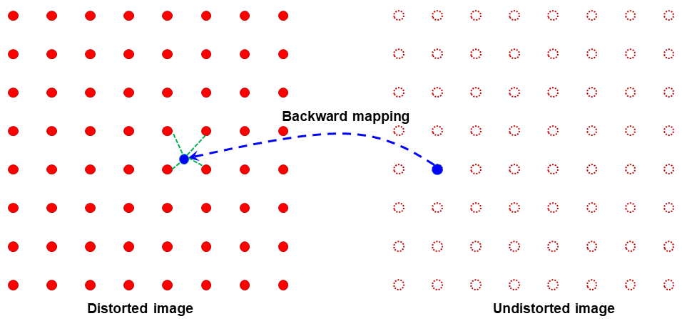
Fig. 2.2.8.1 Demonstration of the backward mapping.
For radial distortion; given \(({x_u}, {y_u})\) , \(({x_{COD}}, {y_{COD}})\), and \((k_0^b, k_1^b,..., k_n^b)\) of a backward model; the correction routine is as follows:
-> Translate the coordinates: \(x_u = x_u - x_{COD}\); \(y_u = y_u - y_{COD}\).
-> Calculate: \(r_u = \sqrt{x_u^2 + y_u^2}\); \(r_d = r_u(k_0^b + {k_1^b}{r_u} + {k_2^b}{r_u^2} + ... + {k_n^b}{r_u^n})\).
-> Calculate: \(x_d = x_u{r_d / r_u}\); \(y_d = y_u{r_d / r_u}\).
-> Translate the coordinates: \(x_d = x_d + x_{COD}\); \(y_d = y_d + y_{COD}\).
-> Find 4 nearest grid points of the distorted image by combing two sets of [floor(\(x_d\)), ceil(\(x_d\))] and [floor(\(y_d\)), ceil(\(y_d\))]. Clip values out of the range of the grid.
-> Interpolate the value at \(({x_d}, {y_d})\) using the values of 4 nearest points. Assign the result to the point \(({x_u}, {y_u})\) in the undistorted image.
Correcting perspective distortion is straightforward. Given \(({x_u}, {y_u})\) and coefficients \((k_1^b, k_2^b,..., k_8^b)\), Eq. (2.2.6.6) (2.2.6.7) are used to calculate \(x_d\), \(y_d\). Then, the image value at this location is calculated by interpolation as explained above.
2.2.9. Summary
The above sections present a complete workflow of calibrating a lens-coupled detector in a concise way. It can be divided into three stages: pre-processing stage is for extracting and grouping reference-points from a calibration image; processing stage is for calculating coefficients of correction models; and post-processing stage is for correcting images. Discorpy’s API is structured following this workflow including input-output and utility modules.
As shown above, parameters of correction models for radial distortion, the distortion center, and perspective distortion can be determined independently by using grid lines of reference points extracted from a single calibration image. This makes Discorpy a practical tool for a wide range of imaging applications. Details on how to use Discorpy to process real data are provided in section 3. New developments [C2] introduced in Discorpy 1.7 for calibrating strong radial distortion (i.e., fisheye distortion) in the presence of perspective distortion using only a single calibration image are presented in section 4.