3.3.2. Process an X-ray target image having perspective effect
The following workflow shows how to use Discorpy to process an X-ray target image, acquired at Beamline I13 Diamond Light Source, which has a small perspective effect.
The following codes load the image, extract reference-points, and group them into lines. Note that the accepted_ratio parameter is adjusted to remove lines have a small number of points. Lines with small number of points can affect the parabolic fit leading to a cascading effect to the accuracy of the correction model.
import numpy as np
import matplotlib.pyplot as plt
import discorpy.losa.loadersaver as losa
import discorpy.prep.preprocessing as prep
import discorpy.proc.processing as proc
import discorpy.post.postprocessing as post

# Initial parameters
file_path = "../../data/dot_pattern_02.jpg"
output_base = "E:/output_demo_02/"
num_coef = 5  # Number of polynomial coefficients
mat0 = losa.load_image(file_path) # Load image
(height, width) = mat0.shape
# Segment dots
mat1 = prep.binarization(mat0)
# Calculate the median dot size and distance between them.
(dot_size, dot_dist) = prep.calc_size_distance(mat1)
# Remove non-dot objects
mat1 = prep.select_dots_based_size(mat1, dot_size)
# Remove non-elliptical objects
mat1 = prep.select_dots_based_ratio(mat1)
losa.save_image(output_base + "/segmented_dots.jpg", mat1)
# Calculate the slopes of horizontal lines and vertical lines.
hor_slope = prep.calc_hor_slope(mat1)
ver_slope = prep.calc_ver_slope(mat1)
# Group points into lines
list_hor_lines = prep.group_dots_hor_lines(mat1, hor_slope, dot_dist, accepted_ratio=0.8)
list_ver_lines = prep.group_dots_ver_lines(mat1, ver_slope, dot_dist, accepted_ratio=0.8)
# Optional: remove outliers
list_hor_lines = prep.remove_residual_dots_hor(list_hor_lines, hor_slope)
list_ver_lines = prep.remove_residual_dots_ver(list_ver_lines, ver_slope)
# Save output for checking
losa.save_plot_image(output_base + "/horizontal_lines.png", list_hor_lines, height, width)
losa.save_plot_image(output_base + "/vertical_lines.png", list_ver_lines, height, width)
list_hor_data = post.calc_residual_hor(list_hor_lines, 0.0, 0.0)
list_ver_data = post.calc_residual_ver(list_ver_lines, 0.0, 0.0)
losa.save_residual_plot(output_base + "/hor_residual_before_correction.png",
                      list_hor_data, height, width)
losa.save_residual_plot(output_base + "/ver_residual_before_correction.png",
                      list_ver_data, height, width)

print("Horizontal slope: {0}. Vertical slope: {1}".format(hor_slope, ver_slope))
#>> Horizontal slope: -0.03194770332102831. Vertical slope: 0.03625649318792672
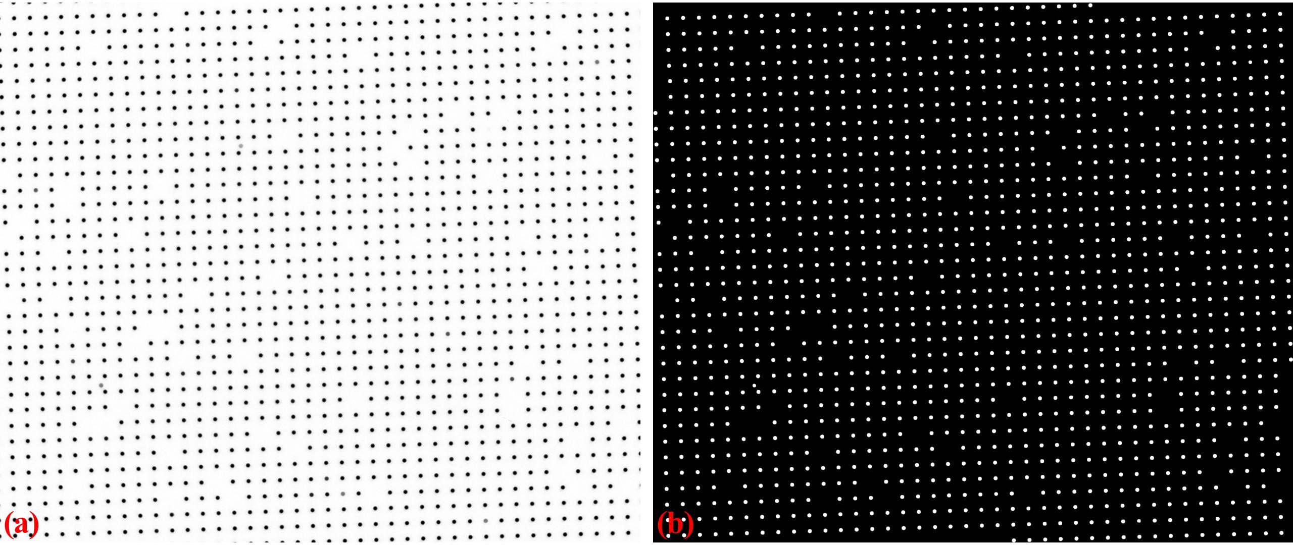
Fig. 3.3.2.1 . (a) X-ray target image. (b) Segmented image.
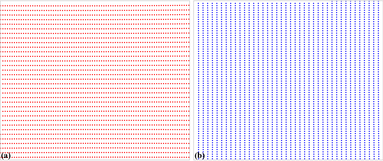
Fig. 3.3.2.2 . (a) Horizontal lines. (b) Vertical lines.
As can be seen from the highlighted output above, the slopes of horizontal lines and vertical lines are quite different, compared to the results in demo 1. This indicates that there is a perspective effect. We can confirm that by plotting coefficients of parabolic fits of lines. Note that the signs of b-coefficients of parabolic fits for horizontal lines are reversed because they use a different axes origin compared to vertical lines.
# Calculate the center of distortion, but just for parabolic fit.
(xcen_tmp, ycen_tmp) = proc.find_cod_bailey(list_hor_lines, list_ver_lines)
# Apply the parabolic fit to lines
list_hor_coef = proc._para_fit_hor(list_hor_lines, xcen_tmp, ycen_tmp)[0]
list_ver_coef = proc._para_fit_ver(list_ver_lines, xcen_tmp, ycen_tmp)[0]
# Plot the results
plt.figure(0)
plt.plot(list_hor_coef[:, 2], list_hor_coef[:, 0], "-o")
plt.plot(list_ver_coef[:, 2], list_ver_coef[:, 0], "-o")
plt.xlabel("c-coefficient")
plt.ylabel("a-coefficient")

plt.figure(1)
plt.plot(list_hor_coef[:, 2], -list_hor_coef[:, 1], "-o")
plt.plot(list_ver_coef[:, 2], list_ver_coef[:, 1], "-o")
plt.xlabel("c-coefficient")
plt.ylabel("b-coefficient")
plt.show()
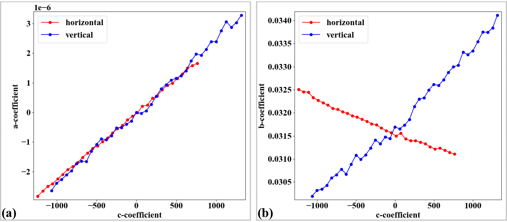
Fig. 3.3.2.3 . (a) Plot of a-coefficients vs c-coefficients of parabolic fits. (b) Plot of b-coefficients vs c-coefficients.
As can be seen in Fig. 3.3.2.3 (b), the slopes are significantly different between two groups of lines. To correct this perspective effect, the coefficients of parabolas are adjusted (Fig. 3.3.2.4) to satisfy the conditions as explained in section 2.2. After that, grid of points are regenerated using these updated coefficients (Fig. 3.3.2.5).
# Correct parabola coefficients
hor_coef_corr, ver_coef_corr = proc._generate_non_perspective_parabola_coef(
                                list_hor_lines, list_ver_lines)[0:2]
# Plot to check the results
plt.figure(0)
plt.plot(hor_coef_corr[:, 2], hor_coef_corr[:, 0], "-o")
plt.plot(ver_coef_corr[:, 2], ver_coef_corr[:, 0], "-o")
plt.xlabel("c-coefficient")
plt.ylabel("a-coefficient")
plt.figure(1)
plt.plot(hor_coef_corr[:, 2], -hor_coef_corr[:, 1], "-o")
plt.plot(ver_coef_corr[:, 2], ver_coef_corr[:, 1], "-o")
plt.xlabel("c-coefficient")
plt.ylabel("b-coefficient")
plt.ylim((0.03, 0.034))
plt.show()
# Regenerate grid points with the correction of perspective effect.
list_hor_lines, list_ver_lines = proc.regenerate_grid_points_parabola(
    list_hor_lines, list_ver_lines, perspective=True)
# Save output for checking
losa.save_plot_image(output_base + "/horizontal_lines_regenerated.png", list_hor_lines,
                   height, width)
losa.save_plot_image(output_base + "/vertical_lines_regenerated.png", list_ver_lines,
                   height, width)
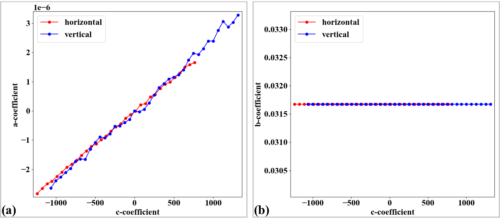
Fig. 3.3.2.4 Parabola coefficients after correction. (a) Plot of a-coefficients vs c-coefficients. (b) Plot of b-coefficients vs c-coefficients.
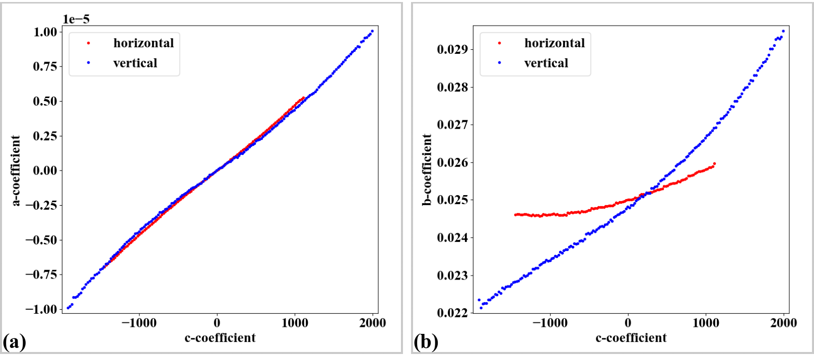
Fig. 3.3.2.5 Grid points regenerated using the updated parabola-coefficients. Note that there are no missing points as compared to Fig. 3.3.2.2. (a) Horizontal lines. (b) Vertical lines.
The rest of the workflow is to calculate the center of distortion and coefficients of the backward model, then unwarp the image. As can be seen in Fig. 3.3.2.7 and Fig. 3.3.2.8, the improvement of the accuracy after correcting the perspective effect is clear.
(xcenter, ycenter) = proc.find_cod_coarse(list_hor_lines, list_ver_lines)
list_fact = proc.calc_coef_backward(list_hor_lines, list_ver_lines,
                                    xcenter, ycenter, num_coef)
losa.save_metadata_txt(output_base + "/coefficients_radial_distortion.txt",
                     xcenter, ycenter, list_fact)
print("X-center: {0}. Y-center: {1}".format(xcenter, ycenter))
print("Coefficients: {0}".format(list_fact))
# Check the correction results:
# Apply correction to the lines of points
list_uhor_lines = post.unwarp_line_backward(list_hor_lines, xcenter, ycenter, list_fact)
list_uver_lines = post.unwarp_line_backward(list_ver_lines, xcenter, ycenter, list_fact)
list_hor_data = post.calc_residual_hor(list_uhor_lines, xcenter, ycenter)
list_ver_data = post.calc_residual_ver(list_uver_lines, xcenter, ycenter)
losa.save_residual_plot(output_base + "/hor_residual_after_correction.png",
                      list_hor_data, height, width)
losa.save_residual_plot(output_base + "/ver_residual_after_correction.png",
                      list_ver_data, height, width)
# Load coefficients from previous calculation if need to
# (xcenter, ycenter, list_fact) = losa.load_metadata_txt(
#     output_base + "/coefficients_radial_distortion.txt")
# Correct the image
corrected_mat = post.unwarp_image_backward(mat0, xcenter, ycenter, list_fact)
# Save results. Note that the output is 32-bit numpy array. Convert to lower-bit if need to.
losa.save_image(output_base + "/corrected_image.tif", corrected_mat)
losa.save_image(output_base + "/difference.tif", corrected_mat - mat0)
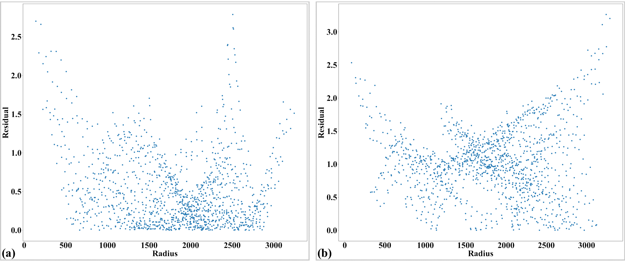
Fig. 3.3.2.6 Residual of the distorted points. The origin of the coordinate system is at the top-left of an image. (a) For horizontal lines. (b) For vertical lines.
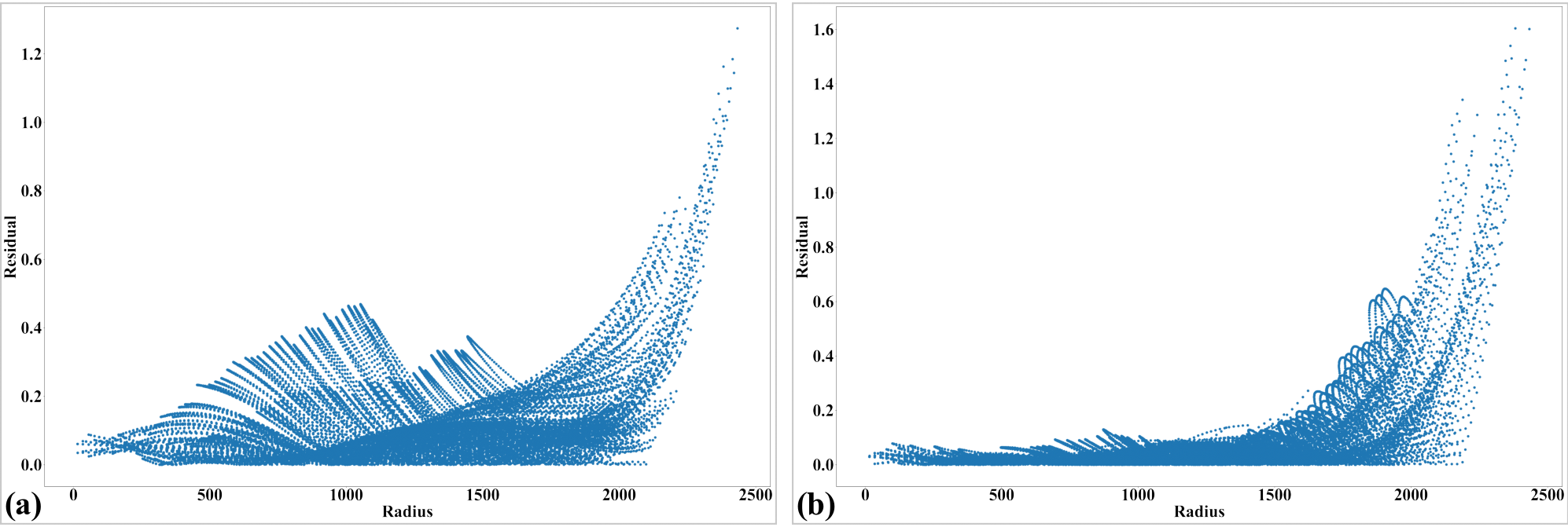
Fig. 3.3.2.7 Residual of the unwarpped points with perspective effect. The origin of the coordinate system is at the center of distortion. (a) For horizontal lines. (b) For vertical lines.
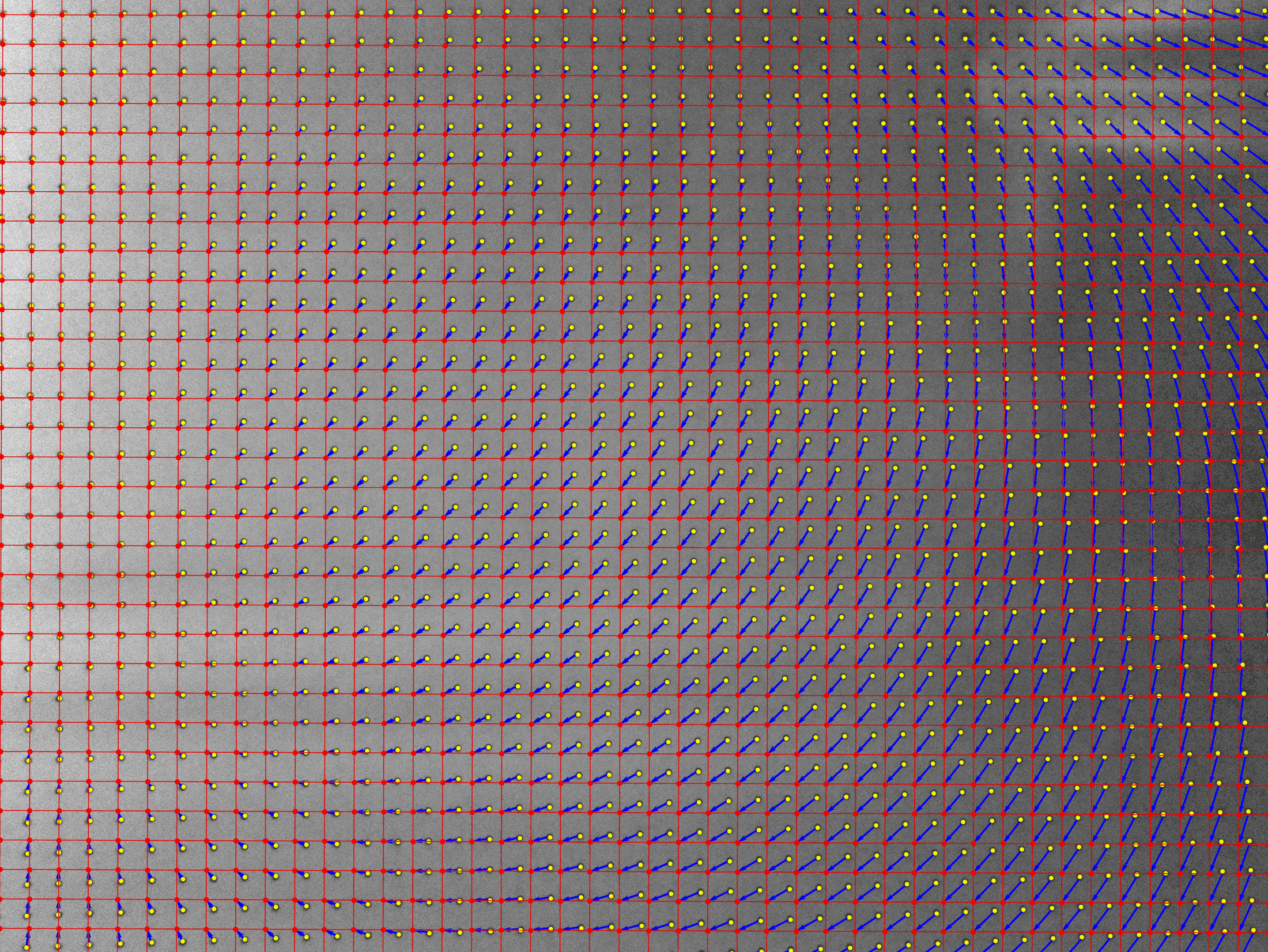
Fig. 3.3.2.8 Residual of the unwarpped points after correcting the perspective effect. (a) For horizontal lines. (b) For vertical lines.

Fig. 3.3.2.9 Difference between images before and after distortion correction.
Click here to download the Python codes.