3.3.3. Process a challenging X-ray target image
Extracting reference-points from an image and grouping them into lines are the most challenging steps in the processing workflow. Calculating coefficients of distortion-correction models is straightforward using Discorpy’s API. The following demo shows how to tweak parameters of pre-processing methods to process a challenging calibration-image which was acquired at Beamline I13, Diamond Light Source.
First of all, the background of the image is corrected to support the step of binarizing the image.
import numpy as np
import discorpy.losa.loadersaver as losa
import discorpy.prep.preprocessing as prep
import discorpy.proc.processing as proc
import discorpy.post.postprocessing as post

# Initial parameters
file_path = "../../data/dot_pattern_04.jpg"
output_base = "E:/output_demo_03/"
num_coef = 5  # Number of polynomial coefficients
mat0 = losa.load_image(file_path)  # Load image
(height, width) = mat0.shape

# Correct non-uniform background.
mat1 = prep.normalization_fft(mat0, sigma=20)
losa.save_image(output_base + "/image_normed.tif", mat1)
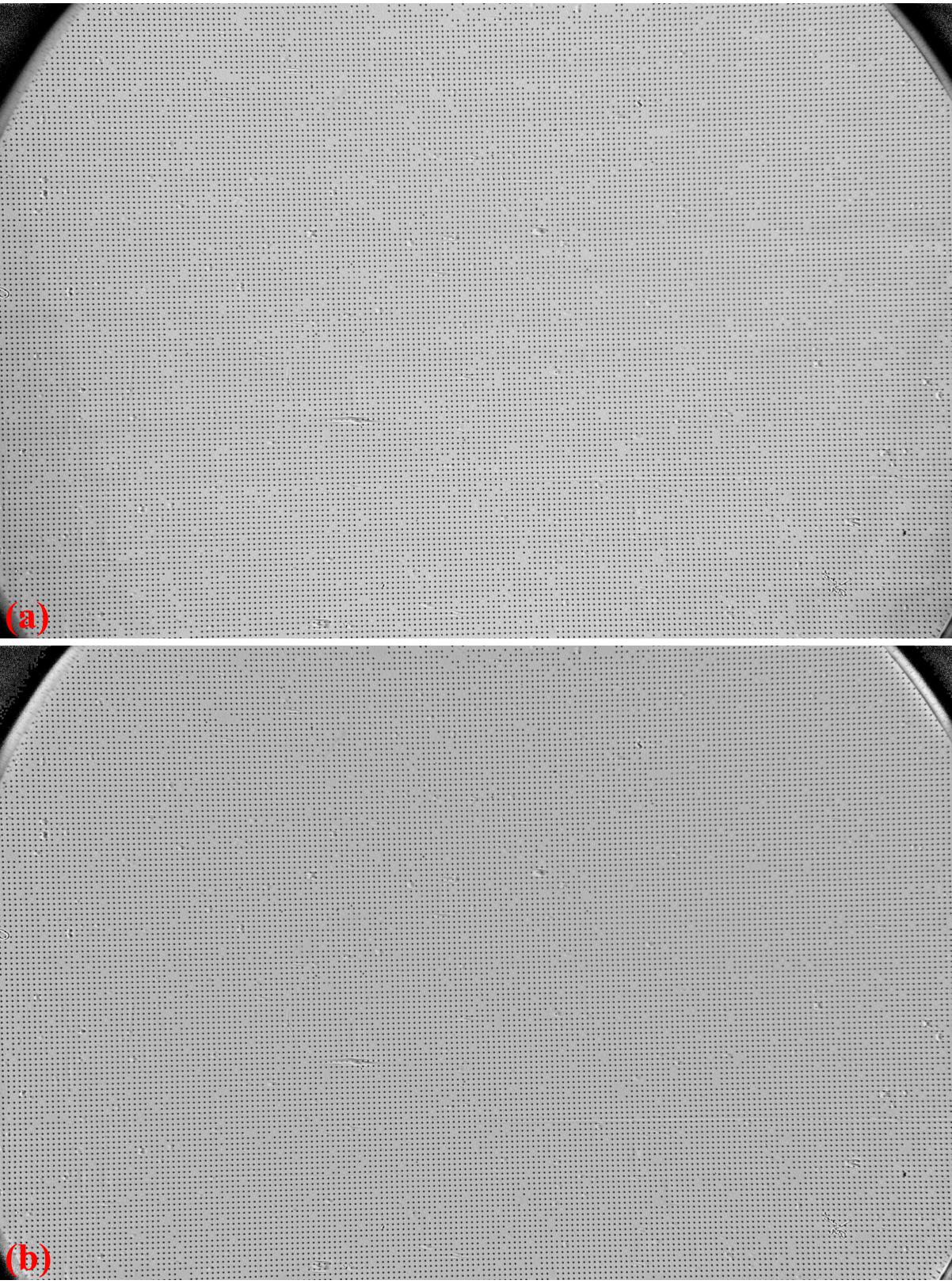
Fig. 3.3.3.1 . (a) X-ray target image. (b) Normalized image.
The binarization method uses the Otsu’s method for calculating the threshold by default. In a case that the calculated value may not work, users can pass a threshold value manually or calculate it by another method.
# Segment dots.
threshold = prep.calculate_threshold(mat1, bgr="bright", snr=3.0)
mat1 = prep.binarization(mat1, ratio=0.5, thres=threshold)
losa.save_image(output_base + "/image_binarized.tif", mat1)
There are lots of non-dot objects left after the binarization step (Fig. 3.3.3.2 (a)). They can be removed further (Fig. 3.3.3.2 (b)) by tweaking parameters of the selection methods. The ratio parameter is increased because there are small binary-dots around the edges of the image.
# Calculate the median dot size and distance between them.
(dot_size, dot_dist) = prep.calc_size_distance(mat1)
# Remove non-dot objects
mat1 = prep.select_dots_based_size(mat1, dot_size, ratio=0.8)
# Remove non-elliptical objects
mat1 = prep.select_dots_based_ratio(mat1, ratio=0.8)
losa.save_image(output_base + "/image_cleaned.tif", mat1)
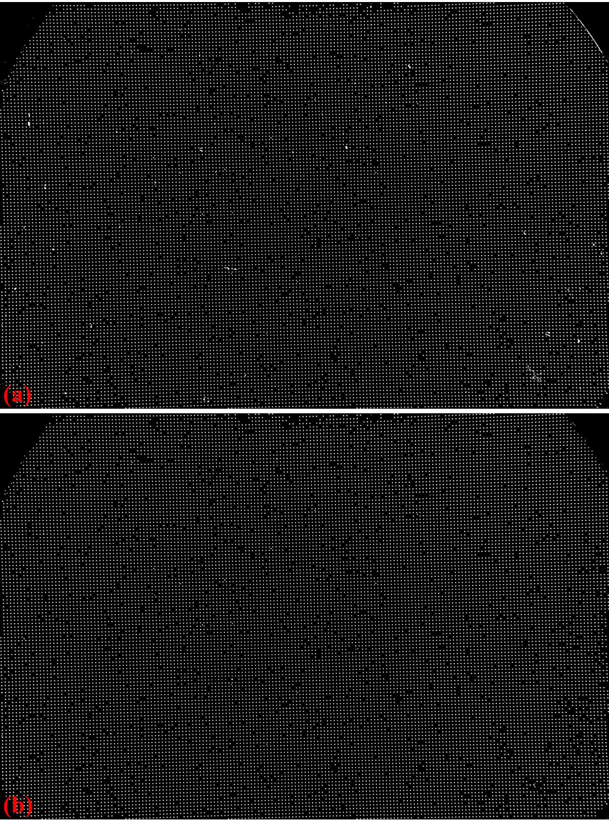
Fig. 3.3.3.2 . (a) Segmented binary objects. (b) Large-size objects removed.
Many of these small binary-objects are not the dots (reference-objects). They can be removed in the grouping step as shown in the codes below and can be seen in Fig. 3.3.3.3. Distortion is strong (Fig. 3.3.3.4).
# Calculate the slopes of horizontal lines and vertical lines.
hor_slope = prep.calc_hor_slope(mat1)
ver_slope = prep.calc_ver_slope(mat1)
print("Horizontal slope: {0}. Vertical slope: {1}".format(hor_slope, ver_slope))

# Group points into lines
list_hor_lines = prep.group_dots_hor_lines(mat1, hor_slope, dot_dist, ratio=0.3,
                                           num_dot_miss=10, accepted_ratio=0.65)
list_ver_lines = prep.group_dots_ver_lines(mat1, ver_slope, dot_dist, ratio=0.3,
                                           num_dot_miss=10, accepted_ratio=0.65)
# Remove outliers
list_hor_lines = prep.remove_residual_dots_hor(list_hor_lines, hor_slope,
                                               residual=2.0)
list_ver_lines = prep.remove_residual_dots_ver(list_ver_lines, ver_slope,
                                               residual=2.0)

# Save output for checking
losa.save_plot_image(output_base + "/horizontal_lines.png", list_hor_lines,
                   height, width)
losa.save_plot_image(output_base + "/vertical_lines.png", list_ver_lines,
                   height, width)
list_hor_data = post.calc_residual_hor(list_hor_lines, 0.0, 0.0)
list_ver_data = post.calc_residual_ver(list_ver_lines, 0.0, 0.0)
losa.save_residual_plot(output_base + "/hor_residual_before_correction.png",
                      list_hor_data, height, width)
losa.save_residual_plot(output_base + "/ver_residual_before_correction.png",
                      list_ver_data, height, width)
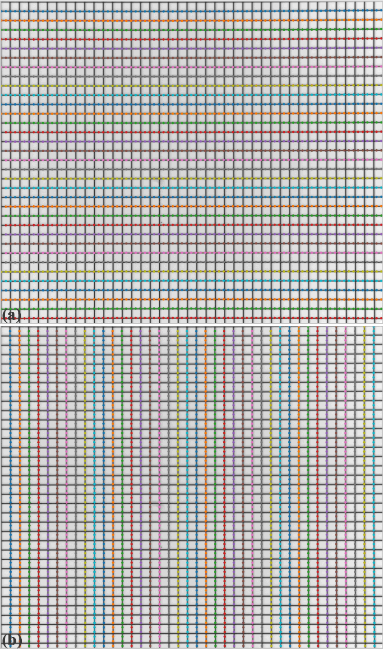
Fig. 3.3.3.3 . (a) Grouped horizontal points. (b) Grouped vertical points.
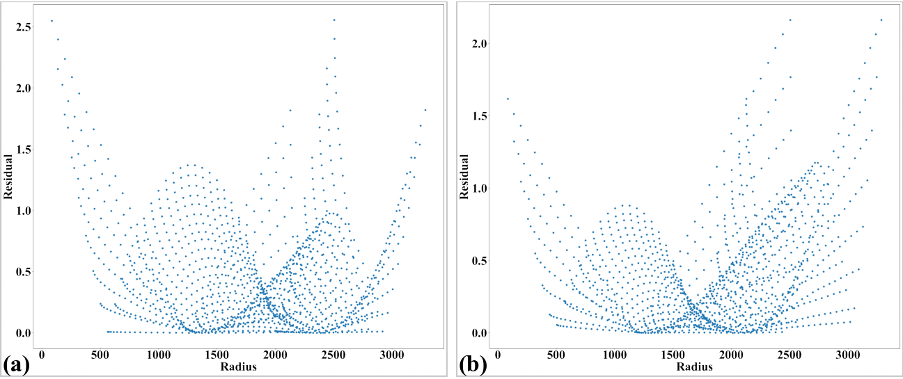
Fig. 3.3.3.4 Residual of the distorted points. The origin of the coordinate system is at the top-left of an image. (a) For horizontal lines. (b) For vertical lines.
There is perspective effect (Fig. 3.3.3.5) caused by the X-ray target was mounted not in parallel to the CCD chip. This can be corrected by a single line of code.
# Regenerate grid points after correcting the perspective effect.
list_hor_lines, list_ver_lines = proc.regenerate_grid_points_parabola(
    list_hor_lines, list_ver_lines, perspective=True)
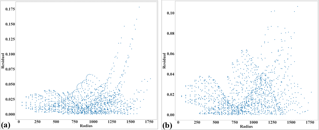
Fig. 3.3.3.5 Impact of the perspective distortion. (a) Plot of a-coefficients vs c-coefficients of parabolic fits. (b) Plot of b-coefficients vs c-coefficients.
The next steps of calculating the center of rotation and coefficients of a polynomial model are straightforward.
# Calculate parameters of the radial correction model
(xcenter, ycenter) = proc.find_cod_coarse(list_hor_lines, list_ver_lines)
list_fact = proc.calc_coef_backward(list_hor_lines, list_ver_lines,
                                    xcenter, ycenter, num_coef)
losa.save_metadata_txt(output_base + "/coefficients_radial_distortion.txt",
                     xcenter, ycenter, list_fact)
print("X-center: {0}. Y-center: {1}".format(xcenter, ycenter))
print("Coefficients: {0}".format(list_fact))
The accuracy of the model is checked by unwarping the lines of points and the image. There are some points with residuals more than 1 pixel near the edges of the image. It can be caused by blurry dots.
# Apply correction to the lines of points
list_uhor_lines = post.unwarp_line_backward(list_hor_lines, xcenter, ycenter,
                                            list_fact)
list_uver_lines = post.unwarp_line_backward(list_ver_lines, xcenter, ycenter,
                                            list_fact)
# Calculate the residual of the unwarpped points.
list_hor_data = post.calc_residual_hor(list_uhor_lines, xcenter, ycenter)
list_ver_data = post.calc_residual_ver(list_uver_lines, xcenter, ycenter)
# Save the results for checking
losa.save_plot_image(output_base + "/unwarpped_horizontal_lines.png",
                   list_uhor_lines, height, width)
losa.save_plot_image(output_base + "/unwarpped_vertical_lines.png",
                   list_uver_lines, height, width)
losa.save_residual_plot(output_base + "/hor_residual_after_correction.png",
                      list_hor_data, height, width)
losa.save_residual_plot(output_base + "/ver_residual_after_correction.png",
                      list_ver_data, height, width)

# Correct the image
corrected_mat = post.unwarp_image_backward(mat0, xcenter, ycenter, list_fact)
# Save results. Note that the output is 32-bit-tif.
losa.save_image(output_base + "/corrected_image.tif", corrected_mat)
losa.save_image(output_base + "/difference.tif", corrected_mat - mat0)
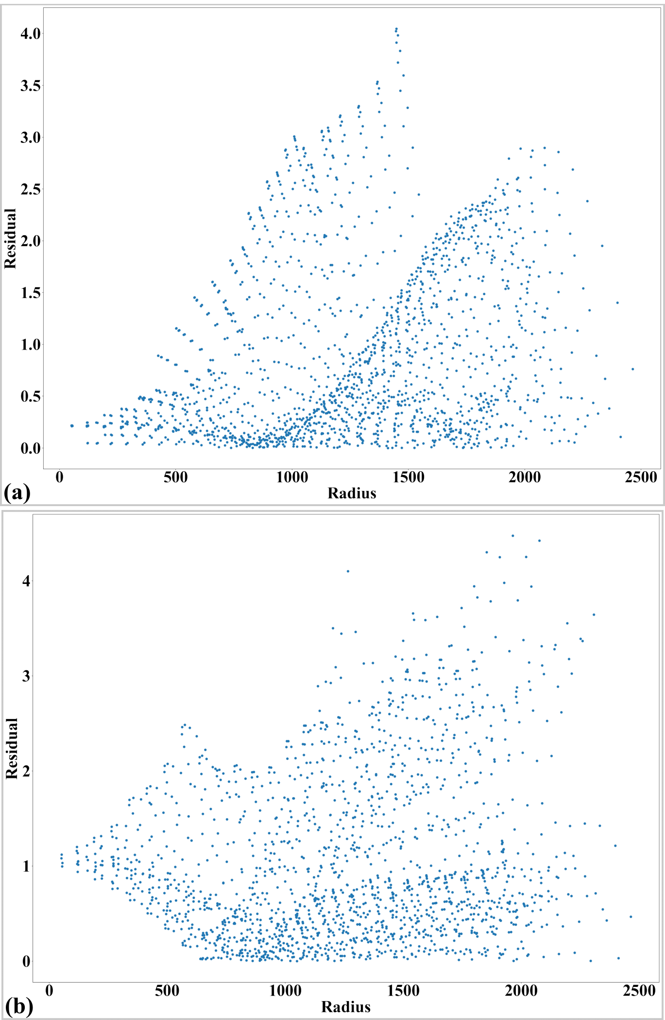
Fig. 3.3.3.6 Unwarped lines of points. Note that these lines are regenerated after the step of correcting perspective effect. (a) Horizontal lines. (b) Vertical lines.
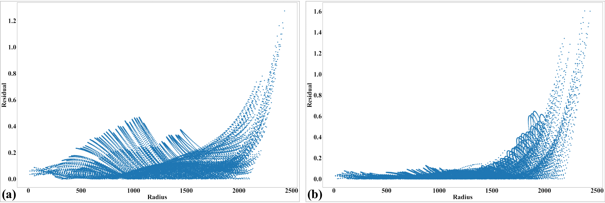
Fig. 3.3.3.7 Residual of the unwarpped points after correcting the perspective effect. (a) For horizontal lines. (b) For vertical lines.
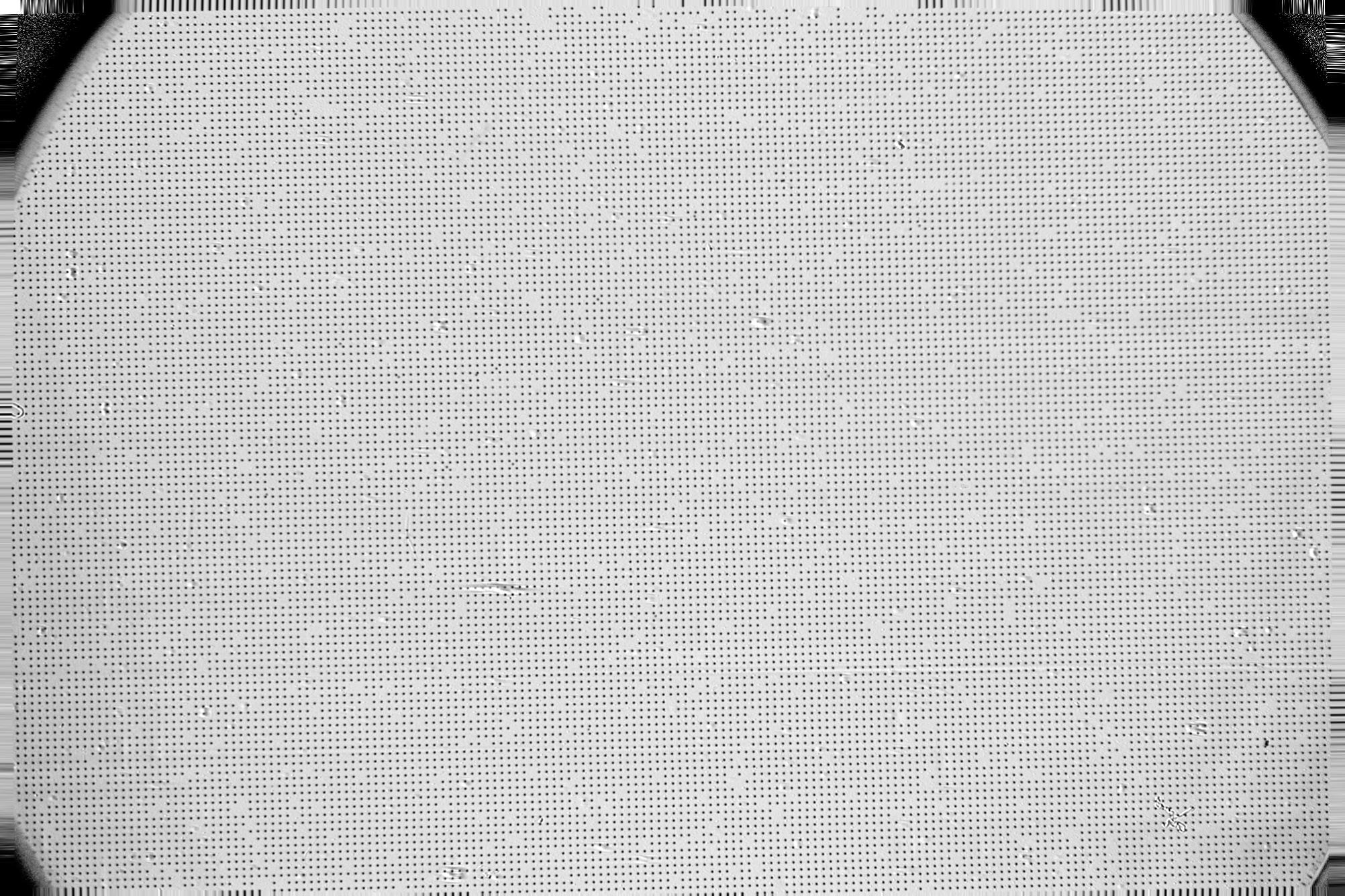
Fig. 3.3.3.8 Unwarped image
Fig. 3.3.3.9 Difference between images before (Fig. 3.3.3.1) and after (Fig. 3.3.3.8) unwarping.
Click here to download the Python codes.