3.3.1. Process a high-quality calibration image
The following workflow shows how to use Discorpy to process a high-quality calibration image acquired at Beamline I12, Diamond Light Source.
Load the image:
import numpy as np
import discorpy.losa.loadersaver as losa
import discorpy.prep.preprocessing as prep
import discorpy.proc.processing as proc
import discorpy.post.postprocessing as post

# Initial parameters
file_path = "../../data/dot_pattern_01.jpg"
output_base = "E:/output_demo_01/"
num_coef = 5  # Number of polynomial coefficients
mat0 = losa.load_image(file_path) # Load image
(height, width) = mat0.shape
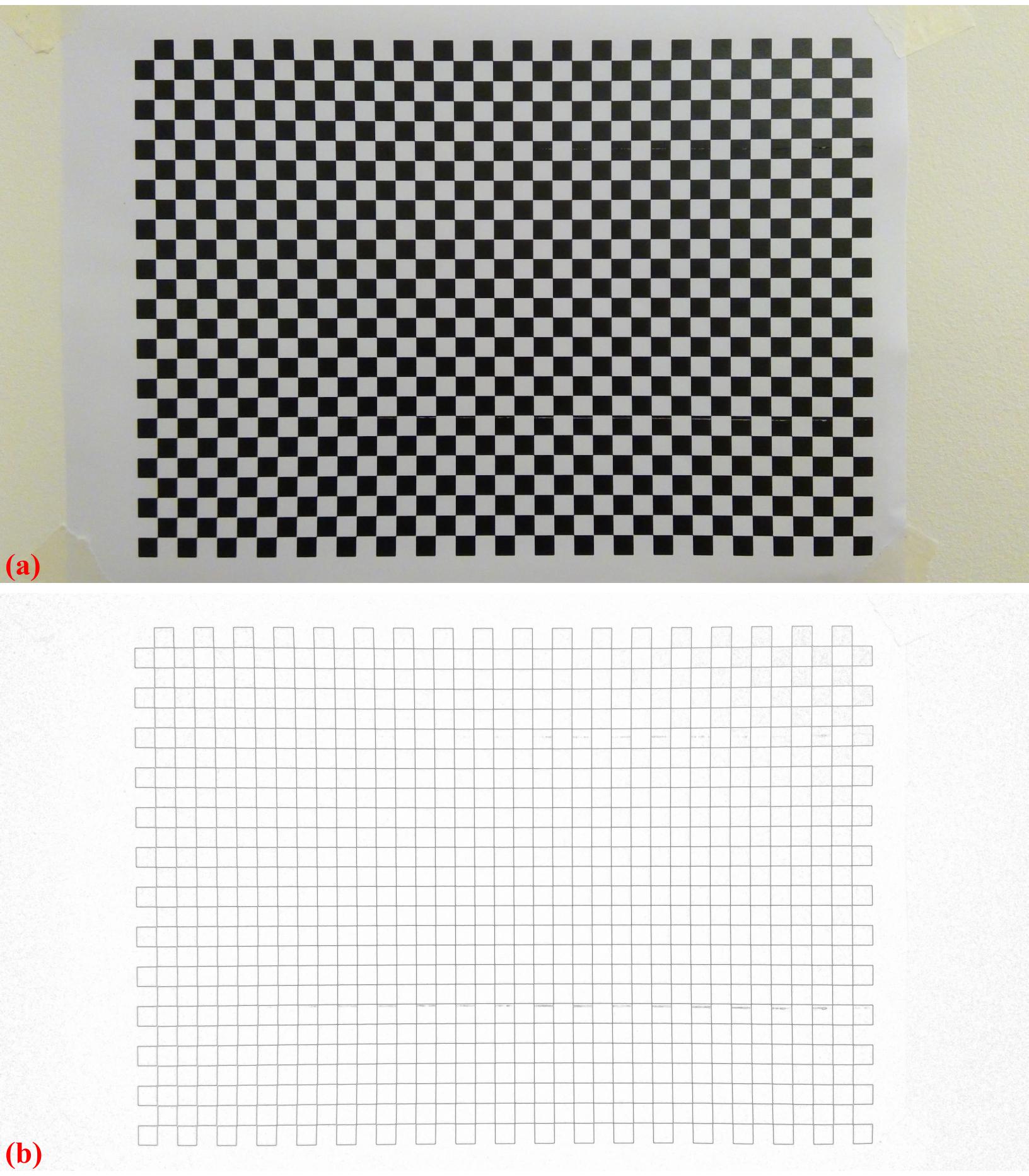
Fig. 3.3.1.1 Visible dot-target.
Extract reference-points:
# Segment dots
mat1 = prep.binarization(mat0)
# Calculate the median dot size and distance between them.
(dot_size, dot_dist) = prep.calc_size_distance(mat1)
# Remove non-dot objects
mat1 = prep.select_dots_based_size(mat1, dot_size)
# Remove non-elliptical objects
mat1 = prep.select_dots_based_ratio(mat1)
losa.save_image(output_base + "/segmented_dots.jpg", mat1) # Save image for checking
# Calculate the slopes of horizontal lines and vertical lines.
hor_slope = prep.calc_hor_slope(mat1)
ver_slope = prep.calc_ver_slope(mat1)
print("Horizontal slope: {0}. Vertical slope {1}".format(hor_slope, ver_slope))

#>> Horizontal slope: 0.01124473800478091. Vertical slope -0.011342266682773354
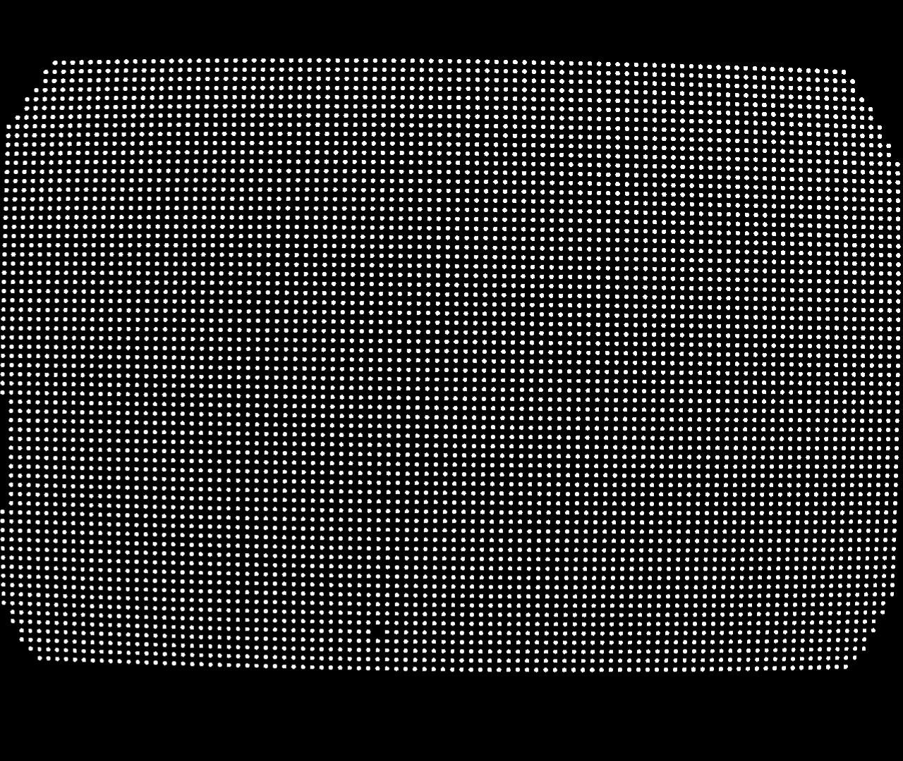
Fig. 3.3.1.2 Segmented dots.
As can be seen from the highlighted output above, the slopes of horizontal lines and vertical lines are nearly the same (note that their signs are opposite due to the use of different origin-axis). This indicates that perspective distortion is negligible. The next step is to group points into lines. After the grouping step, perspective effect; if there is; can be corrected simply by adding a single line of command.
# Group points to horizontal lines
list_hor_lines = prep.group_dots_hor_lines(mat1, hor_slope, dot_dist)
# Group points to vertical lines
list_ver_lines = prep.group_dots_ver_lines(mat1, ver_slope, dot_dist)
# Optional: remove horizontal outliers
list_hor_lines = prep.remove_residual_dots_hor(list_hor_lines, hor_slope)
# Optional: remove vertical outliers
list_ver_lines = prep.remove_residual_dots_ver(list_ver_lines, ver_slope)
# Save output for checking
losa.save_plot_image(output_base + "/horizontal_lines.png", list_hor_lines, height, width)
losa.save_plot_image(output_base + "/vertical_lines.png", list_ver_lines, height, width)

# Optional: correct perspective effect. Only available from Discorpy 1.4
# list_hor_lines, list_ver_lines = proc.regenerate_grid_points_parabola(
#                      list_hor_lines, list_ver_lines, perspective=True)
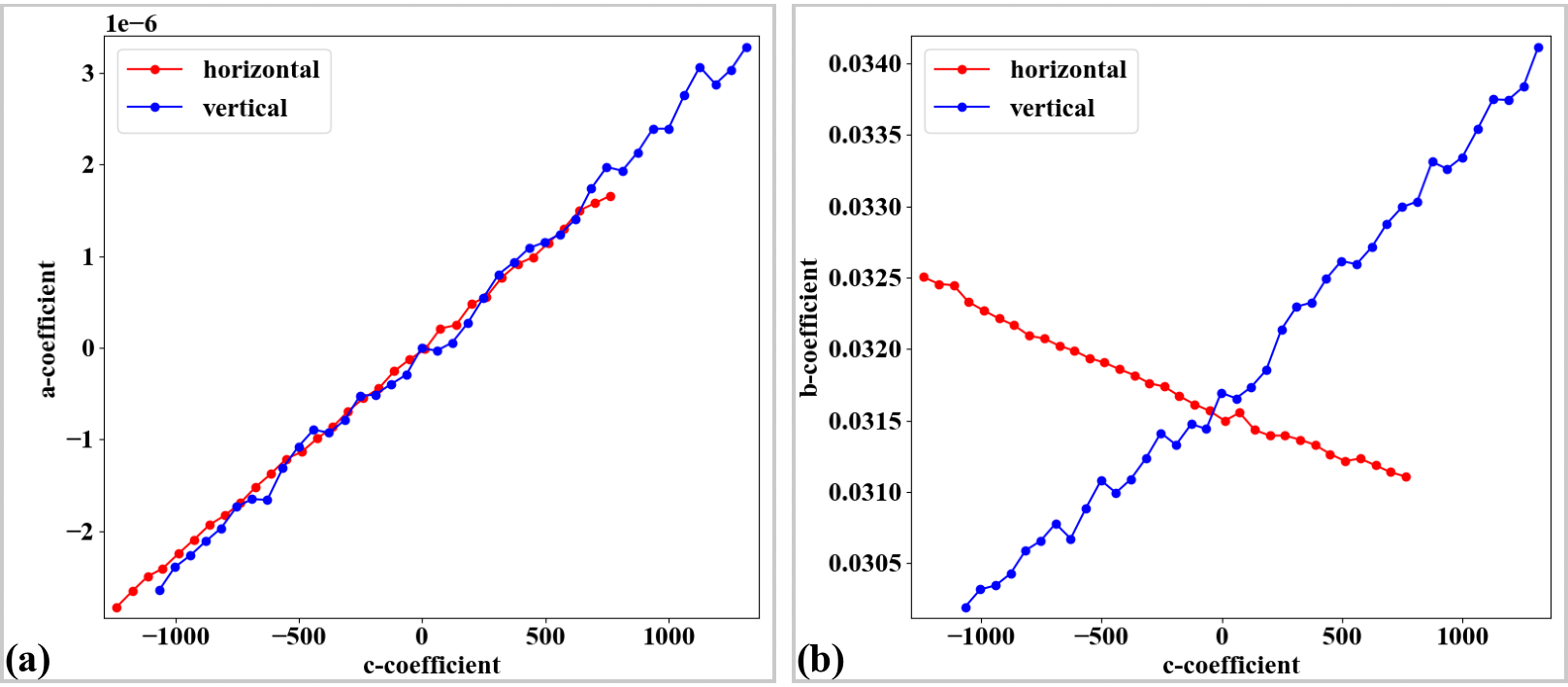
Fig. 3.3.1.3 Reference-points (center-of-mass of dots) after grouped into horizontal lines (a) and vertical lines (b).
We can check the straightness of lines of points by calculating the distances of the grouped points to their fitted straight lines. This helps to assess if the distortion is significant or not. Note that the origin of the coordinate system before distortion correction is at the top-left corner of an image.
list_hor_data = post.calc_residual_hor(list_hor_lines, 0.0, 0.0)
list_ver_data = post.calc_residual_ver(list_ver_lines, 0.0, 0.0)
losa.save_residual_plot(output_base + "/hor_residual_before_correction.png",
                      list_hor_data, height, width)
losa.save_residual_plot(output_base + "/ver_residual_before_correction.png",
                      list_ver_data, height, width)
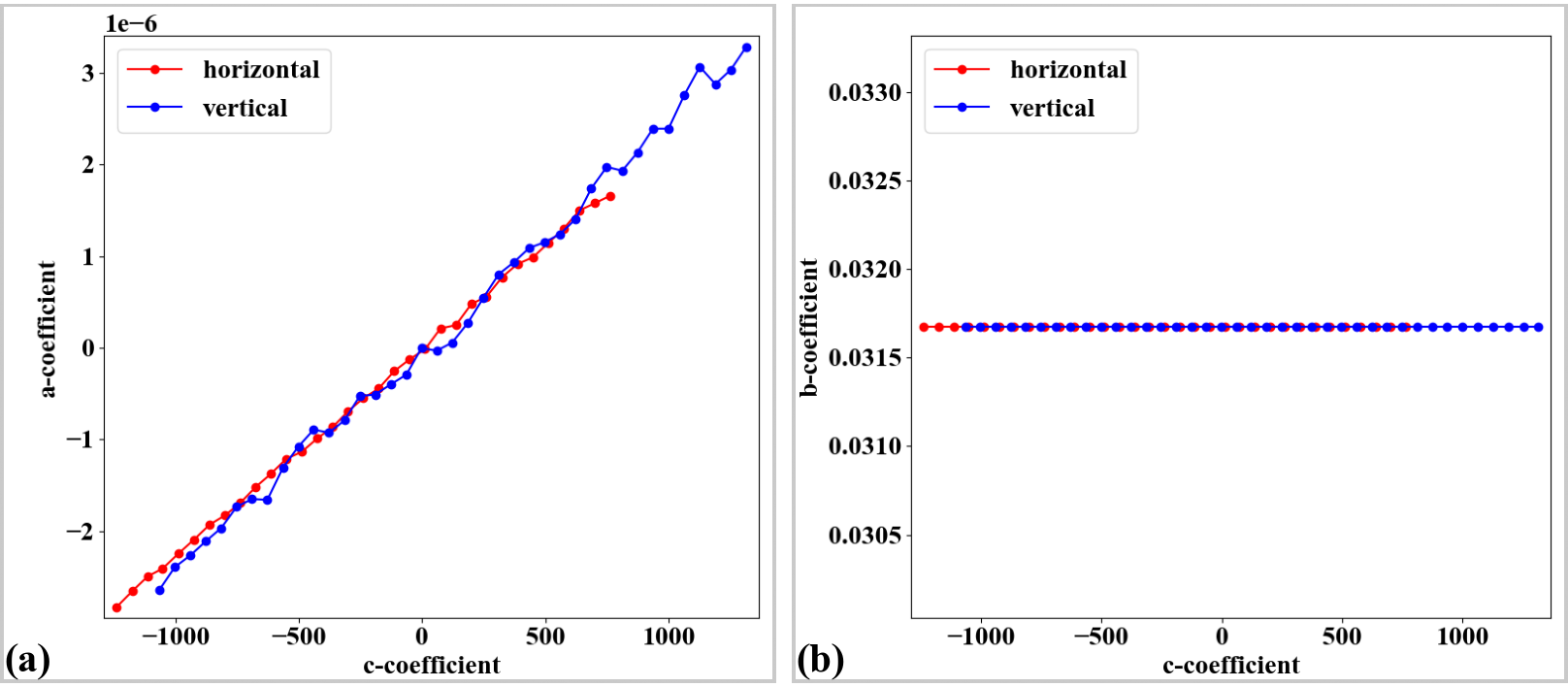
Fig. 3.3.1.4 Plot of the distances of the dot-centroids from their fitted straight line against their distances from the axes origin. (a) For horizontal lines. (b) For vertical lines.
As shown in Fig. 3.3.1.4, the residual is more than 12 pixels which means that distortion is significant and needs to be corrected. The next step is to calculate the center of distortion (COD) and the coefficients of the backward mapping for a radial distortion model.
# Calculate the center of distortion
(xcenter, ycenter) = proc.find_cod_coarse(list_hor_lines, list_ver_lines)
# Calculate coefficients of the correction model
list_fact = proc.calc_coef_backward(list_hor_lines, list_ver_lines,
                                    xcenter, ycenter, num_coef)
# Save the results for later use.
losa.save_metadata_txt(output_base + "/coefficients_radial_distortion.txt",
                     xcenter, ycenter, list_fact)
print("X-center: {0}. Y-center: {1}".format(xcenter, ycenter))
print("Coefficients: {0}".format(list_fact))
"""
>> X-center: 1252.1528590042283. Y-center: 1008.9088499595639
>> Coefficients: [1.00027631e+00, -1.25730878e-06, -1.43170401e-08,
                  -1.65727563e-12, 7.89109870e-16]
"""
Using the determined parameters of the correction model, we can unwarp the lines of points and check the correction results.
# Apply correction to the lines of points
list_uhor_lines = post.unwarp_line_backward(list_hor_lines, xcenter, ycenter,
                                            list_fact)
list_uver_lines = post.unwarp_line_backward(list_ver_lines, xcenter, ycenter,
                                            list_fact)
# Save the results for checking
losa.save_plot_image(output_base + "/unwarpped_horizontal_lines.png", list_uhor_lines,
                   height, width)
losa.save_plot_image(output_base + "/unwarpped_vertical_lines.png", list_uver_lines,
                   height, width)
# Calculate the residual of the unwarpped points.
list_hor_data = post.calc_residual_hor(list_uhor_lines, xcenter, ycenter)
list_ver_data = post.calc_residual_ver(list_uver_lines, xcenter, ycenter)
# Save the results for checking
losa.save_residual_plot(output_base + "/hor_residual_after_correction.png",
                      list_hor_data, height, width)
losa.save_residual_plot(output_base + "/ver_residual_after_correction.png",
                      list_ver_data, height, width)
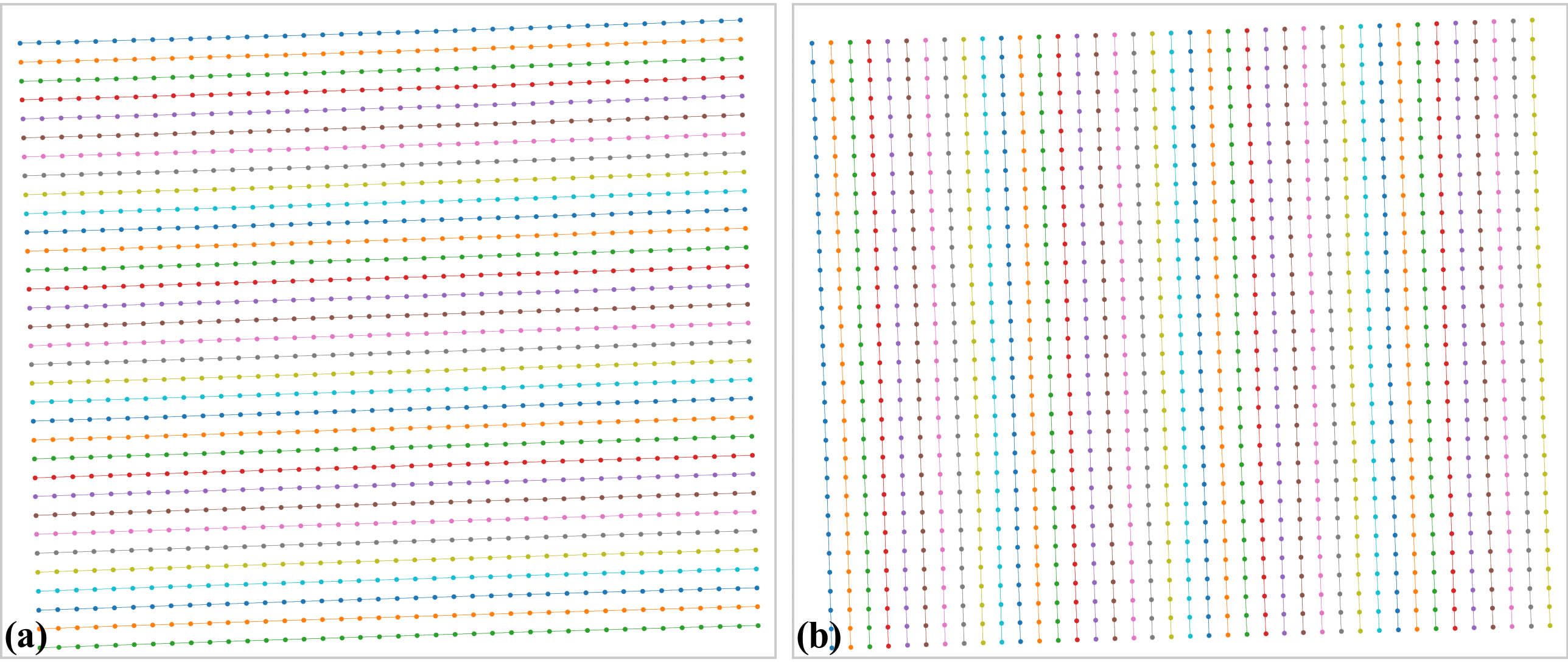
Fig. 3.3.1.5 . (a) Unwarpped horizontal lines. (b) Unwarpped vertical lines.

Fig. 3.3.1.6 Residual of the unwarpped points. Note that the origin of the coordinate system is at the center of distortion. (a) For horizontal lines. (b) For vertical lines.
As can be seen from Fig. 3.3.1.6 the accuracy of the correction results is sub-pixel. The last step of the workflow is to use the determined model for correcting images.
# Load coefficients from previous calculation if need to
# (xcenter, ycenter, list_fact) = losa.load_metadata_txt(
#     output_base + "/coefficients_radial_distortion.txt")
# Correct the image
corrected_mat = post.unwarp_image_backward(mat0, xcenter, ycenter, list_fact)
# Save results. Note that the output is 32-bit numpy array. Convert to lower-bit if need to.
losa.save_image(output_base + "/corrected_image.tif", corrected_mat)
losa.save_image(output_base + "/difference.tif", corrected_mat - mat0)
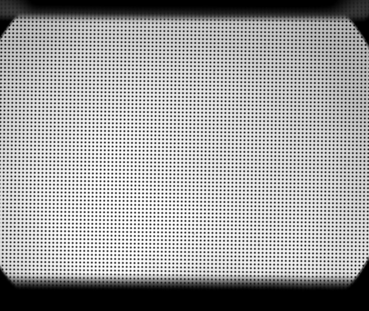
Fig. 3.3.1.7 Corrected image.
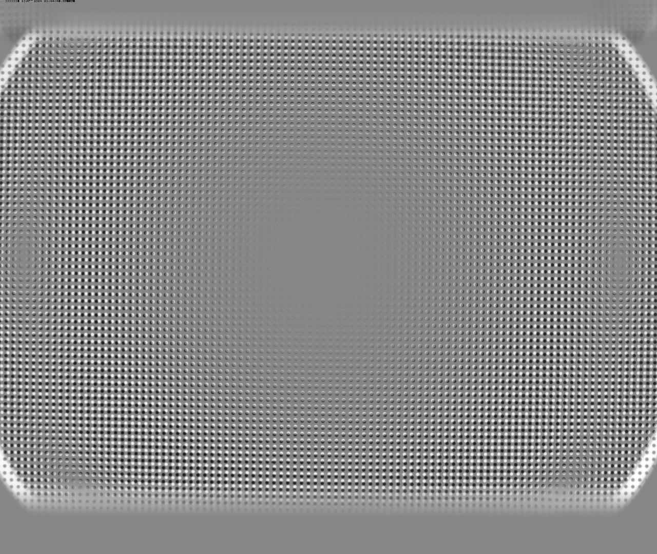
Fig. 3.3.1.8 Difference between images before (Fig. 3.3.1.1) and after (Fig. 3.3.1.7) the correction.
Click here to download the Python codes.