3.3.6. Calibrate a camera using a chessboard image
The following workflow shows how to calibrate a commercial camera using a chessboard image. First of all, the chessboard pattern was created using this website. The generated pattern was printed and stuck to a flat wall (Fig. 3.3.6.1). Then, its image was taken using the front-facing camera of a Microsoft Surface Pro Laptop. The pincushion distortion is visible in the image.
Load the chessboard image, convert to a line-pattern image.
import numpy as np
import discorpy.losa.loadersaver as losa
import discorpy.prep.preprocessing as prep
import discorpy.prep.linepattern as lprep
import discorpy.proc.processing as proc
import discorpy.post.postprocessing as post

# Initial parameters
file_path = "../../data/laptop_camera/chessboard.jpg"
output_base = "E:/output_demo_06/"
num_coef = 5  # Number of polynomial coefficients
mat0 = losa.load_image(file_path) # Load image
(height, width) = mat0.shape

# Convert the chessboard image to a line-pattern image
mat1 = lprep.convert_chessboard_to_linepattern(mat0)
losa.save_image(output_base + "/line_pattern_converted.jpg", mat1)

# Calculate slope and distance between lines
slope_hor, dist_hor = lprep.calc_slope_distance_hor_lines(mat1, radius=15, sensitive=0.5)
slope_ver, dist_ver = lprep.calc_slope_distance_ver_lines(mat1, radius=15, sensitive=0.5)
print("Horizontal slope: ", slope_hor, " Distance: ", dist_hor)
print("Vertical slope: ", slope_ver, " Distance: ", dist_ver)
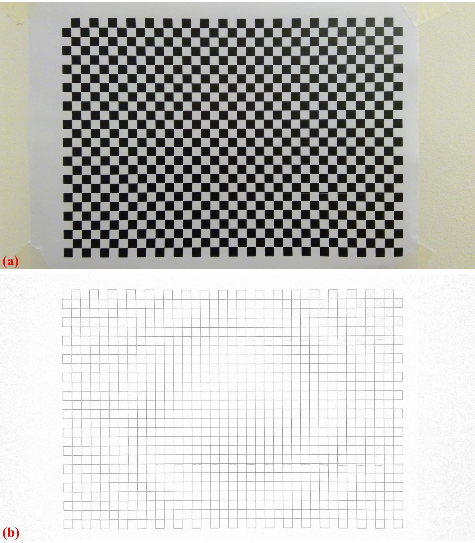
Fig. 3.3.6.1 . (a) Chessboard image. (b) Line-pattern image generated from image (a).
Extract reference-points (adjust parameters: radius and/or sensitive if need to). Note that users can use other methods available in Scikit-image to perform this step directly on the chessboard image. There are many unwanted points (Fig. 3.3.6.2) but they can be removed by the grouping method (Fig. 3.3.6.3) in Discorpy.
# Extract reference-points
list_points_hor_lines = lprep.get_cross_points_hor_lines(mat1, slope_ver, dist_ver,
                                                         ratio=0.3, norm=True, offset=450,
                                                         bgr="bright", radius=15,
                                                         sensitive=0.5, denoise=True,
                                                         subpixel=True)
list_points_ver_lines = lprep.get_cross_points_ver_lines(mat1, slope_hor, dist_hor,
                                                         ratio=0.3, norm=True, offset=150,
                                                         bgr="bright", radius=15,
                                                         sensitive=0.5, denoise=True,
                                                         subpixel=True)
if len(list_points_hor_lines) == 0 or len(list_points_ver_lines) == 0:
    raise ValueError("No reference-points detected !!! Please adjust parameters !!!")
losa.save_plot_points(output_base + "/ref_points_horizontal.png", list_points_hor_lines,
                    height, width, color="red")
losa.save_plot_points(output_base + "/ref_points_vertical.png", list_points_ver_lines,
                    height, width, color="blue")

# Group points into lines
list_hor_lines = prep.group_dots_hor_lines(list_points_hor_lines, slope_hor, dist_hor,
                                           ratio=0.1, num_dot_miss=2, accepted_ratio=0.8)
list_ver_lines = prep.group_dots_ver_lines(list_points_ver_lines, slope_ver, dist_ver,
                                           ratio=0.1, num_dot_miss=2, accepted_ratio=0.8)

# Remove residual dots
list_hor_lines = prep.remove_residual_dots_hor(list_hor_lines, slope_hor, 2.0)
list_ver_lines = prep.remove_residual_dots_ver(list_ver_lines, slope_ver, 2.0)

# Save output for checking
losa.save_plot_image(output_base + "/horizontal_lines.png", list_hor_lines, height, width)
losa.save_plot_image(output_base + "/vertical_lines.png", list_ver_lines, height, width)
list_hor_data = post.calc_residual_hor(list_hor_lines, 0.0, 0.0)
list_ver_data = post.calc_residual_ver(list_ver_lines, 0.0, 0.0)
losa.save_residual_plot(output_base + "/hor_residual_before_correction.png",
                      list_hor_data, height, width)
losa.save_residual_plot(output_base + "/ver_residual_before_correction.png",
                      list_ver_data, height, width)
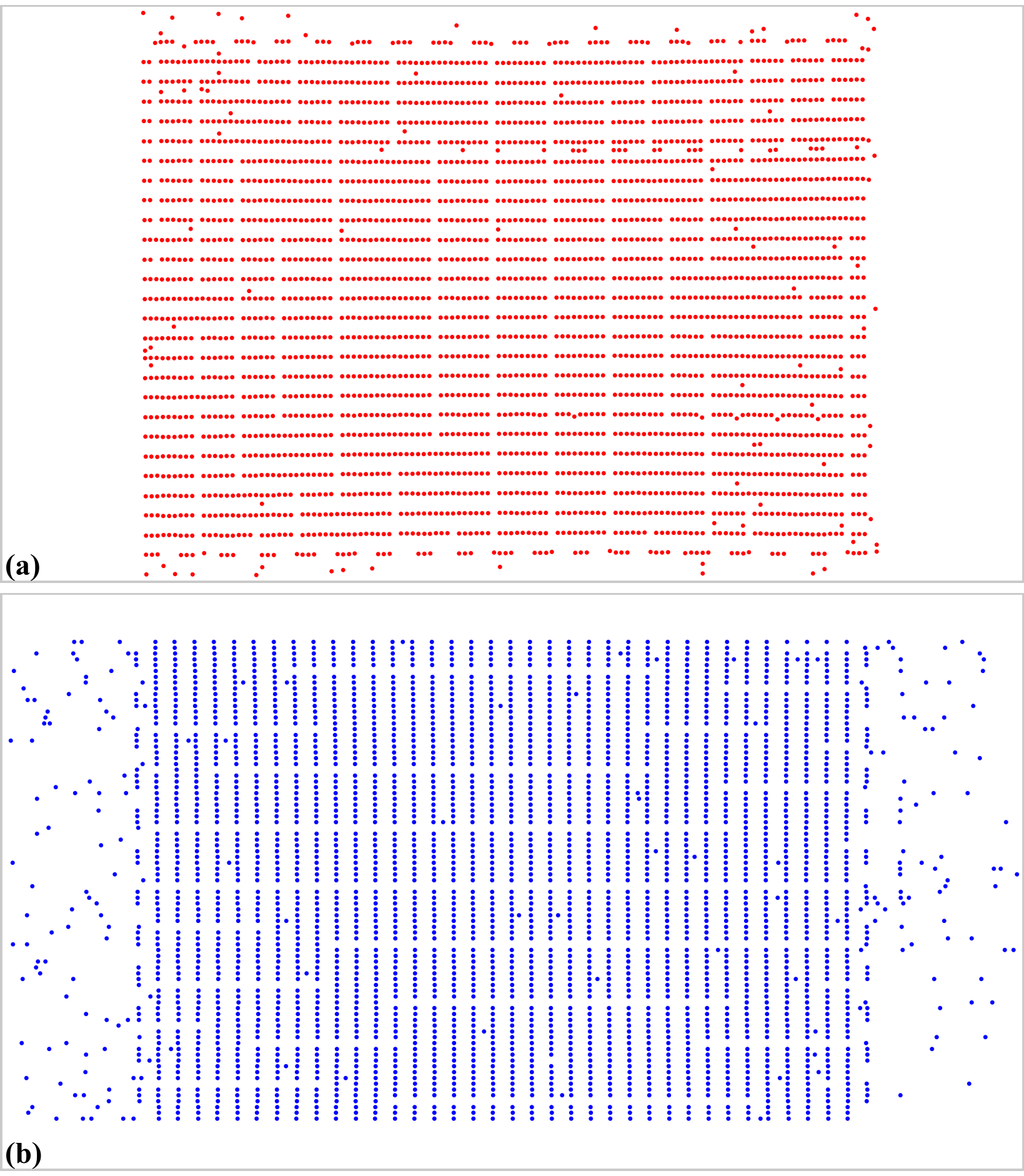
Fig. 3.3.6.2 Extracted reference points from Fig. 3.3.6.1 (b). (a) For horizontal lines. (b) For vertical lines.
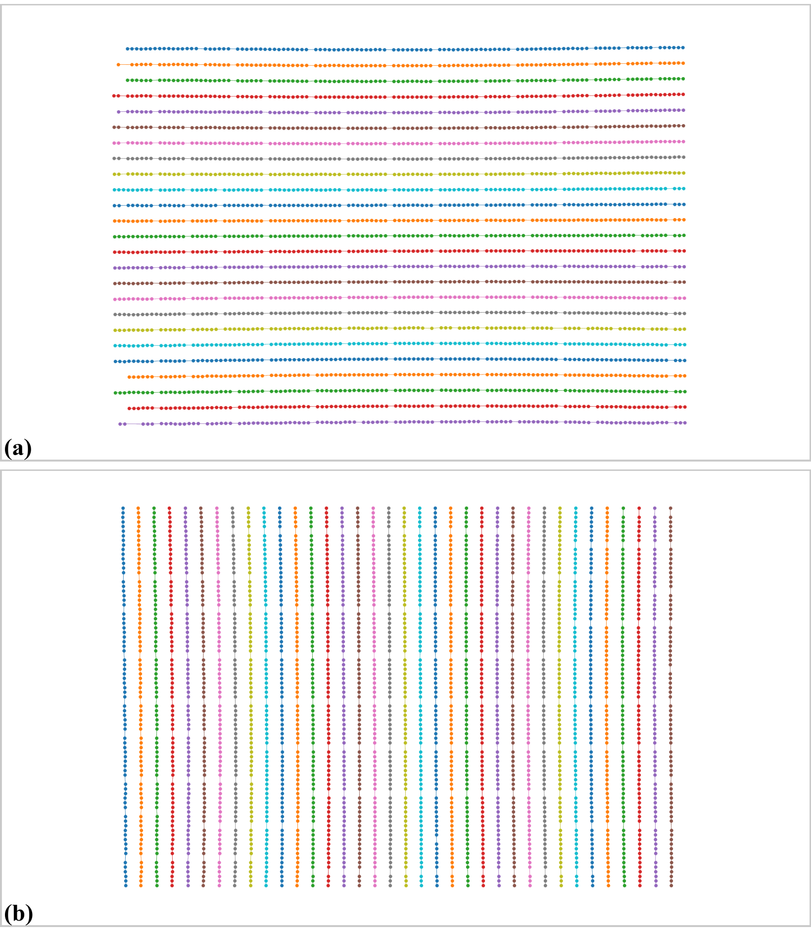
Fig. 3.3.6.3 Grouped points. (a) Horizontal lines. (b) Vertical lines.
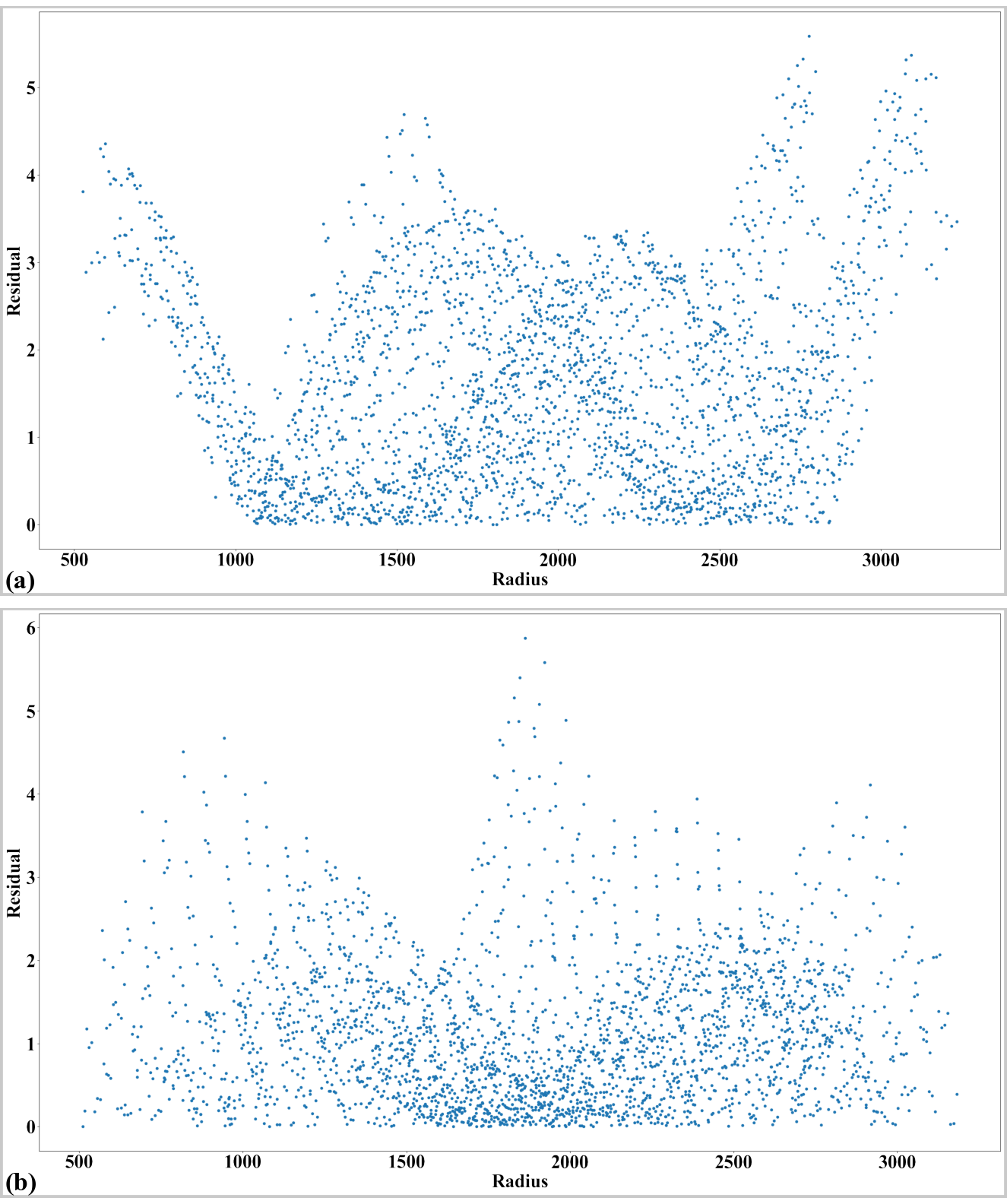
Fig. 3.3.6.4 Residual of distorted points. (a) Horizontal lines. (b) Vertical lines.
Next steps are straightforward. Coefficients of the radial-distortion model are calculated where the perspective effect is corrected before that. The results of applying the model for unwarping lines and images can be seen in Fig. 3.3.6.5 and Fig. 3.3.6.6
# Regenerate grid points after correcting the perspective effect.
list_hor_lines, list_ver_lines = proc.regenerate_grid_points_parabola(
    list_hor_lines, list_ver_lines, perspective=True)

# Calculate parameters of the radial correction model
(xcenter, ycenter) = proc.find_cod_coarse(list_hor_lines, list_ver_lines)
list_fact = proc.calc_coef_backward(list_hor_lines, list_ver_lines,
                                    xcenter, ycenter, num_coef)
losa.save_metadata_txt(output_base + "/coefficients_radial_distortion.txt",
                     xcenter, ycenter, list_fact)
print("X-center: {0}. Y-center: {1}".format(xcenter, ycenter))
print("Coefficients: {0}".format(list_fact))

# Check the correction results:
# Apply correction to the lines of points
list_uhor_lines = post.unwarp_line_backward(list_hor_lines, xcenter, ycenter,
                                            list_fact)
list_uver_lines = post.unwarp_line_backward(list_ver_lines, xcenter, ycenter,
                                            list_fact)
# Calculate the residual of the unwarpped points.
list_hor_data = post.calc_residual_hor(list_uhor_lines, xcenter, ycenter)
list_ver_data = post.calc_residual_ver(list_uver_lines, xcenter, ycenter)
# Save the results for checking
losa.save_plot_image(output_base + "/unwarpped_horizontal_lines.png",
                   list_uhor_lines, height, width)
losa.save_plot_image(output_base + "/unwarpped_vertical_lines.png",
                   list_uver_lines, height, width)
losa.save_residual_plot(output_base + "/hor_residual_after_correction.png",
                      list_hor_data, height, width)
losa.save_residual_plot(output_base + "/ver_residual_after_correction.png",
                      list_ver_data, height, width)
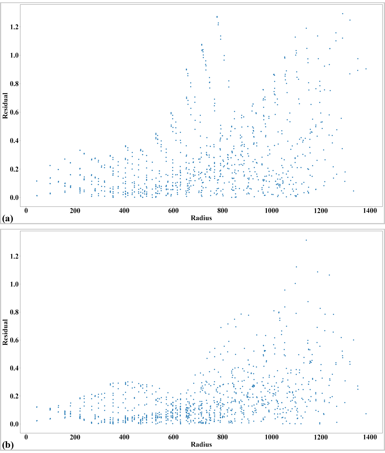
Fig. 3.3.6.5 Residual of unwarped points. (a) Horizontal lines. (b) Vertical lines.
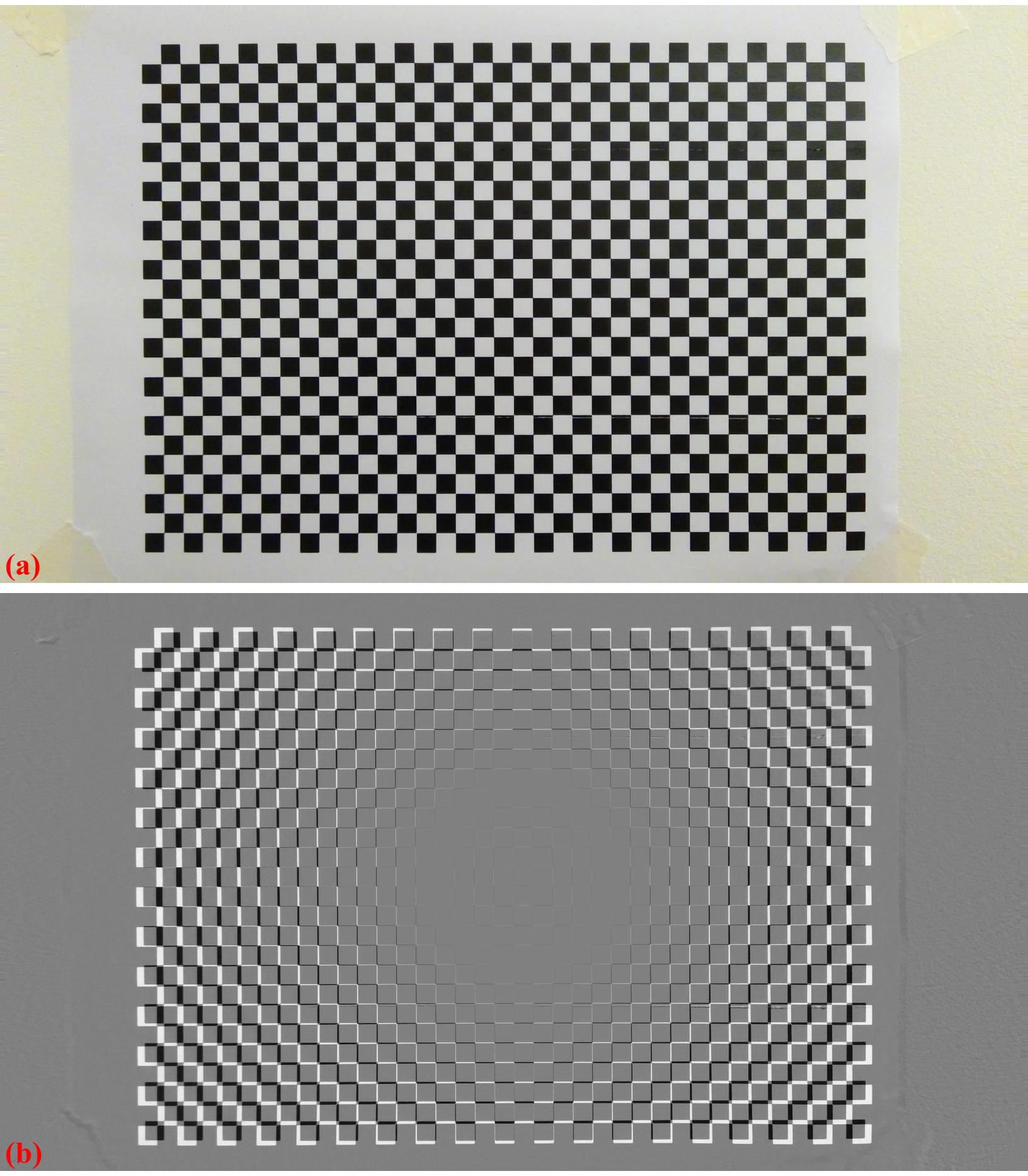
Fig. 3.3.6.6 . (a) Unwarped image of Fig. 3.3.6.1 (a). (b) Difference between the images before and after unwarping.
Calculated coefficients of the correction model can be used to unwarp another image taken by the same camera as demonstrated in Fig. 3.3.6.7. For a color image, we have to correct each channel of the image.
# Load coefficients from previous calculation
(xcenter, ycenter, list_fact) = losa.load_metadata_txt(
    output_base + "/coefficients_radial_distortion.txt")

# Load an image and correct it.
img = losa.load_image("../../data/laptop_camera/test_image.jpg", average=False)
img_corrected = np.copy(img)
for i in range(img.shape[-1]):
    img_corrected[:, :, i] = post.unwarp_image_backward(img[:, :, i], xcenter,
                                                        ycenter, list_fact)
losa.save_image(output_base + "/test_image_corrected.jpg", img_corrected)
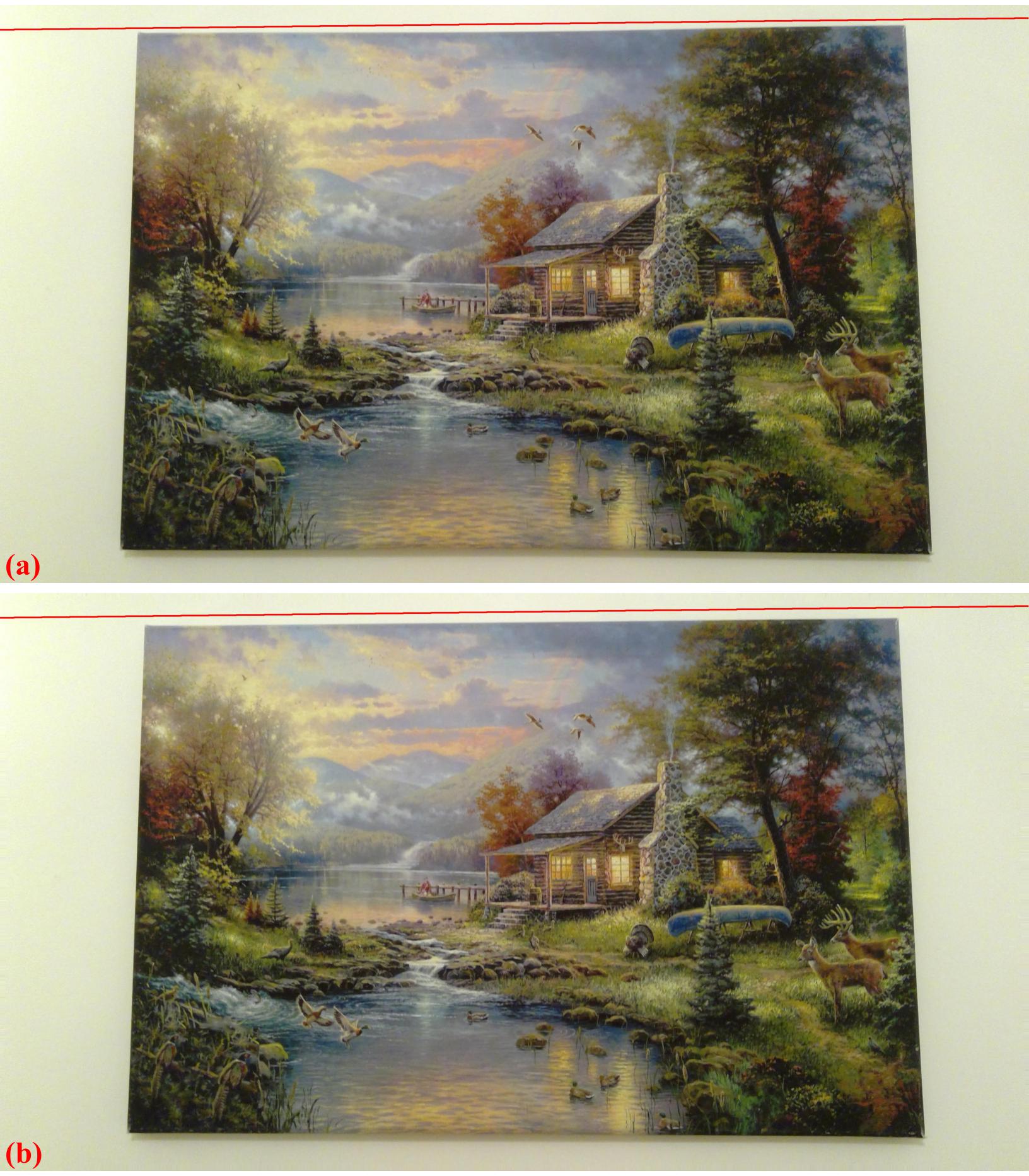
Fig. 3.3.6.7 . (a) Test image taken from the same camera. (b) Unwarped image. The red straight line is added for reference.
Click here to download the Python codes.